- Foreword
- Preface
- Chapter 1. Meet Hadoop
- Chapter 2. MapReduce
- Chapter 3. The Hadoop Distributed Filesystem
- The Design of HDFS
- HDFS Concepts
- The Command-Line Interface
- Hadoop Filesystems
- The Java Interface
- Data Flow
- Parallel Copying with distcp
- Chapter 4. YARN
- Chapter 5. Hadoop I/O
- Data Integrity
- Compression
- Serialization
- File-Based Data Structures
- Chapter 6. Developing a MapReduce Application
- Chapter 7. How MapReduce Works
Hadoop: The Definitive Guide
Tom White
For Eliane, Emilia, and Lottie
Foreword
Doug Cutting, April 2009
Shed in the Yard, California
Hadoop got its start in Nutch. A few of us were attempting to build an open source web search engine and having trouble managing computations running on even a handful of computers. Once Google published its GFS and MapReduce papers, the route became clear. They’d devised systems to solve precisely the problems we were having with Nutch. So we started, two of us, half-time, to try to re-create these systems as a part of Nutch.
We managed to get Nutch limping along on 20 machines, but it soon became clear that to handle the Web’s massive scale, we’d need to run it on thousands of machines, and moreover, that the job was bigger than two half-time developers could handle.
Around that time, Yahoo! got interested, and quickly put together a team that I joined. We split off the distributed computing part of Nutch, naming it Hadoop. With the help of Yahoo!, Hadoop soon grew into a technology that could truly scale to the Web.
In 2006, Tom White started contributing to Hadoop. I already knew Tom through an excellent article he’d written about Nutch, so I knew he could present complex ideas in clear prose. I soon learned that he could also develop software that was as pleasant to read as his prose.
From the beginning, Tom’s contributions to Hadoop showed his concern for users and for the project. Unlike most open source contributors, Tom is not primarily interested in tweaking the system to better meet his own needs, but rather in making it easier for anyone to use.
Initially, Tom specialized in making Hadoop run well on Amazon’s EC2 and S3 services.
Then he moved on to tackle a wide variety of problems, including improving the
MapReduce APIs, enhancing the website, and devising an object serialization framework.
In all cases, Tom presented his ideas precisely. In short order, Tom earned the role of Hadoop committer and soon thereafter became a member of the Hadoop Project Management Committee.
Tom is now a respected senior member of the Hadoop developer community. Though he’s an expert in many technical corners of the project, his specialty is making Hadoop easier to use and understand.
Given this, I was very pleased when I learned that Tom intended to write a book about
Hadoop. Who could be better qualified? Now you have the opportunity to learn about Hadoop from a master — not only of the technology, but also of common sense and plain talk.
Preface
Martin Gardner, the mathematics and science writer, once said in an interview:
Beyond calculus, I am lost. That was the secret of my column’s success. It took me so long to understand what I was writing about that I knew how to write in a way most readers would understand.[1]
In many ways, this is how I feel about Hadoop. Its inner workings are complex, resting as they do on a mixture of distributed systems theory, practical engineering, and common sense. And to the uninitiated, Hadoop can appear alien.
But it doesn’t need to be like this. Stripped to its core, the tools that Hadoop provides for working with big data are simple. If there’s a common theme, it is about raising the level of abstraction — to create building blocks for programmers who have lots of data to store and analyze, and who don’t have the time, the skill, or the inclination to become distributed systems experts to build the infrastructure to handle it.
With such a simple and generally applicable feature set, it seemed obvious to me when I started using it that Hadoop deserved to be widely used. However, at the time (in early 2006), setting up, configuring, and writing programs to use Hadoop was an art. Things have certainly improved since then: there is more documentation, there are more examples, and there are thriving mailing lists to go to when you have questions. And yet the biggest hurdle for newcomers is understanding what this technology is capable of, where it excels, and how to use it. That is why I wrote this book.
The Apache Hadoop community has come a long way. Since the publication of the first edition of this book, the Hadoop project has blossomed. “Big data” has become a household term.2] In this time, the software has made great leaps in adoption, performance, reliability, scalability, and manageability. The number of things being built and run on the Hadoop platform has grown enormously. In fact, it’s difficult for one person to keep track. To gain even wider adoption, I believe we need to make Hadoop even easier to use. This will involve writing more tools; integrating with even more systems; and writing new, improved APIs. I’m looking forward to being a part of this, and I hope this book will encourage and enable others to do so, too.
Administrative Notes
During discussion of a particular Java class in the text, I often omit its package name to reduce clutter. If you need to know which package a class is in, you can easily look it up in the Java API documentation for Hadoop (linked to from the Apache Hadoop home page), or the relevant project. Or if you’re using an integrated development environment (IDE), its auto-complete mechanism can help find what you’re looking for.
Similarly, although it deviates from usual style guidelines, program listings that import multiple classes from the same package may use the asterisk wildcard character to save space (for example, import org.apache.hadoop.io.).
The sample programs in this book are available for download from the book’s website. You will also find instructions there for obtaining the datasets that are used in examples throughout the book, as well as further notes for running the programs in the book and links to updates, additional resources, and my blog.
What’s New in the Fourth Edition?
The fourth edition covers Hadoop 2 exclusively. The Hadoop 2 release series is the current active release series and contains the most stable versions of Hadoop.
There are new chapters covering YARN (Chapter 4), Parquet (Chapter 13), Flume (Chapter 14), Crunch (Chapter 18), and Spark (Chapter 19). There’s also a new section to help readers navigate different pathways through the book (What’s in This Book?).
This edition includes two new case studies (Chapters 22 and 23): one on how Hadoop is used in healthcare systems, and another on using Hadoop technologies for genomics data processing. Case studies from the previous editions can now be found online.
Many corrections, updates, and improvements have been made to existing chapters to bring them up to date with the latest releases of Hadoop and its related projects.
What’s New in the Third Edition?
The third edition covers the 1.x (formerly 0.20) release series of Apache Hadoop, as well as the newer 0.22 and 2.x (formerly 0.23) series. With a few exceptions, which are noted in the text, all the examples in this book run against these versions.
This edition uses the new MapReduce API for most of the examples. Because the old API is still in widespread use, it continues to be discussed in the text alongside the new API, and the equivalent code using the old API can be found on the book’s website.
The major change in Hadoop 2.0 is the new MapReduce runtime, MapReduce 2, which is built on a new distributed resource management system called YARN. This edition includes new sections covering MapReduce on YARN: how it works (Chapter 7) and how to run it (Chapter 10).
There is more MapReduce material, too, including development practices such as packaging MapReduce jobs with Maven, setting the user’s Java classpath, and writing tests with MRUnit (all in Chapter 6). In addition, there is more depth on features such as output committers and the distributed cache (both in Chapter 9), as well as task memory monitoring (Chapter 10). There is a new section on writing MapReduce jobs to process Avro data (Chapter 12), and one on running a simple MapReduce workflow in Oozie (Chapter 6).
The chapter on HDFS (Chapter 3) now has introductions to high availability, federation, and the new WebHDFS and HttpFS filesystems.
The chapters on Pig, Hive, Sqoop, and ZooKeeper have all been expanded to cover the new features and changes in their latest releases.
In addition, numerous corrections and improvements have been made throughout the book.
*What’s New in the Second Edition?
The second edition has two new chapters on Sqoop and Hive (Chapters 15 and 17, respectively), a new section covering Avro (in Chapter 12), an introduction to the new security features in Hadoop (in Chapter 10), and a new case study on analyzing massive network graphs using Hadoop.
This edition continues to describe the 0.20 release series of Apache Hadoop, because this was the latest stable release at the time of writing. New features from later releases are occasionally mentioned in the text, however, with reference to the version that they were introduced in.
Conventions Used in This Book
The following typographical conventions are used in this book:
Italic
Indicates new terms, URLs, email addresses, filenames, and file extensions.
Constant width
Used for program listings, as well as within paragraphs to refer to commands and command-line options and to program elements such as variable or function names, databases, data types, environment variables, statements, and keywords.
Constant width bold
Shows commands or other text that should be typed literally by the user.
Constant width italic
Shows text that should be replaced with user-supplied values or by values determined by context.
Using Code Examples
Supplemental material (code, examples, exercise, etc.) is available for download at this book’s website and on GitHub.
This book is here to help you get your job done. In general, you may use the code in this book in your programs and documentation. You do not need to contact us for permission unless you’re reproducing a significant portion of the code. For example, writing a program that uses several chunks of code from this book does not require permission. Selling or distributing a CD-ROM of examples from O’Reilly books does require permission. Answering a question by citing this book and quoting example code does not require permission. Incorporating a significant amount of example code from this book into your product’s documentation does require permission.
We appreciate, but do not require, attribution. An attribution usually includes the title, author, publisher, and ISBN. For example: “Hadoop: The Definitive Guide, Fourth Edition, by Tom White (O’Reilly). Copyright 2015 Tom White, 978-1-491-90163-2.”
If you feel your use of code examples falls outside fair use or the permission given here, feel free to contact us at permissions@oreilly.com.
Safari® Books Online

Technology professionals, software developers, web designers, and business and creative professionals use Safari Books Online as their primary resource for research, problem solving, learning, and certification training.
Safari Books Online offers a range of plans and pricing for enterprise, government, education, and individuals.
Members have access to thousands of books, training videos, and prepublication manuscripts in one fully searchable database from publishers like O’Reilly Media,
Prentice Hall Professional, Addison-Wesley Professional, Microsoft Press, Sams, Que,
Peachpit Press, Focal Press, Cisco Press, John Wiley & Sons, Syngress, Morgan
Kaufmann, IBM Redbooks, Packt, Adobe Press, FT Press, Apress, Manning, New Riders, McGraw-Hill, Jones & Bartlett, Course Technology, and hundreds more. For more information about Safari Books Online, please visit us online.
How to Contact Us
Please address comments and questions concerning this book to the publisher:
O’Reilly Media, Inc.
1005 Gravenstein Highway North
Sebastopol, CA 95472
800-998-9938 (in the United States or Canada)
707-829-0515 (international or local)
707-829-0104 (fax)
We have a web page for this book, where we list errata, examples, and any additional information. You can access this page at http://bit.ly/hadoop_tdg_4e.
To comment or ask technical questions about this book, send email to bookquestions@oreilly.com.
For more information about our books, courses, conferences, and news, see our website at http://www.oreilly.com.
Find us on Facebook: http://facebook.com/oreilly
Follow us on Twitter: http://twitter.com/oreillymedia
Watch us on YouTube: http://www.youtube.com/oreillymedia
Acknowledgments
I have relied on many people, both directly and indirectly, in writing this book. I would like to thank the Hadoop community, from whom I have learned, and continue to learn, a great deal.
In particular, I would like to thank Michael Stack and Jonathan Gray for writing the chapter on HBase. Thanks also go to Adrian Woodhead, Marc de Palol, Joydeep Sen Sarma, Ashish Thusoo, Andrzej Białecki, Stu Hood, Chris K. Wensel, and Owen O’Malley for contributing case studies.
I would like to thank the following reviewers who contributed many helpful suggestions and improvements to my drafts: Raghu Angadi, Matt Biddulph, Christophe Bisciglia,
Ryan Cox, Devaraj Das, Alex Dorman, Chris Douglas, Alan Gates, Lars George, Patrick
Hunt, Aaron Kimball, Peter Krey, Hairong Kuang, Simon Maxen, Olga Natkovich,
Benjamin Reed, Konstantin Shvachko, Allen Wittenauer, Matei Zaharia, and Philip Zeyliger. Ajay Anand kept the review process flowing smoothly. Philip (“flip”) Kromer kindly helped me with the NCDC weather dataset featured in the examples in this book. Special thanks to Owen O’Malley and Arun C. Murthy for explaining the intricacies of the MapReduce shuffle to me. Any errors that remain are, of course, to be laid at my door.
For the second edition, I owe a debt of gratitude for the detailed reviews and feedback from Jeff Bean, Doug Cutting, Glynn Durham, Alan Gates, Jeff Hammerbacher, Alex Kozlov, Ken Krugler, Jimmy Lin, Todd Lipcon, Sarah Sproehnle, Vinithra Varadharajan, and Ian Wrigley, as well as all the readers who submitted errata for the first edition. I would also like to thank Aaron Kimball for contributing the chapter on Sqoop, and Philip (“flip”) Kromer for the case study on graph processing.
For the third edition, thanks go to Alejandro Abdelnur, Eva Andreasson, Eli Collins, Doug
Cutting, Patrick Hunt, Aaron Kimball, Aaron T. Myers, Brock Noland, Arvind Prabhakar, Ahmed Radwan, and Tom Wheeler for their feedback and suggestions. Rob Weltman kindly gave very detailed feedback for the whole book, which greatly improved the final manuscript. Thanks also go to all the readers who submitted errata for the second edition.
For the fourth edition, I would like to thank Jodok Batlogg, Meghan Blanchette, Ryan
Blue, Jarek Jarcec Cecho, Jules Damji, Dennis Dawson, Matthew Gast, Karthik Kambatla,
Julien Le Dem, Brock Noland, Sandy Ryza, Akshai Sarma, Ben Spivey, Michael Stack, Kate Ting, Josh Walter, Josh Wills, and Adrian Woodhead for all of their invaluable review feedback. Ryan Brush, Micah Whitacre, and Matt Massie kindly contributed new case studies for this edition. Thanks again to all the readers who submitted errata.
I am particularly grateful to Doug Cutting for his encouragement, support, and friendship, and for contributing the Foreword.
Thanks also go to the many others with whom I have had conversations or email discussions over the course of writing the book.
Halfway through writing the first edition of this book, I joined Cloudera, and I want to thank my colleagues for being incredibly supportive in allowing me the time to write and to get it finished promptly.
I am grateful to my editors, Mike Loukides and Meghan Blanchette, and their colleagues at O’Reilly for their help in the preparation of this book. Mike and Meghan have been there throughout to answer my questions, to read my first drafts, and to keep me on schedule.
Finally, the writing of this book has been a great deal of work, and I couldn’t have done it without the constant support of my family. My wife, Eliane, not only kept the home going, but also stepped in to help review, edit, and chase case studies. My daughters, Emilia and Lottie, have been very understanding, and I’m looking forward to spending lots more time with all of them.
[1] Alex Bellos, “The science of fun,” The Guardian, May 31, 2008.
[2] It was added to the Oxford English Dictionary in 2013.
Part I. Hadoop Fundamentals
Chapter 1. Meet Hadoop
In pioneer days they used oxen for heavy pulling, and when one ox couldn’t budge a log, they didn’t try to grow a larger ox. We shouldn’t be trying for bigger computers, but for more systems of computers.
— Grace Hopper
Data!
We live in the data age. It’s not easy to measure the total volume of data stored electronically, but an IDC estimate put the size of the “digital universe” at 4.4 zettabytes in
2013 and is forecasting a tenfold growth by 2020 to 44 zettabytes.3] A zettabyte is 10bytes, or equivalently one thousand exabytes, one million petabytes, or one billion terabytes. That’s more than one disk drive for every person in the world.
This flood of data is coming from many sources. Consider the following:4] The New York Stock Exchange generates about 4−5 terabytes of data per day.
Facebook hosts more than 240 billion photos, growing at 7 petabytes per month.
Ancestry.com, the genealogy site, stores around 10 petabytes of data.
The Internet Archive stores around 18.5 petabytes of data.
The Large Hadron Collider near Geneva, Switzerland, produces about 30 petabytes of data per year.
So there’s a lot of data out there. But you are probably wondering how it affects you. Most of the data is locked up in the largest web properties (like search engines) or in scientific or financial institutions, isn’t it? Does the advent of big data affect smaller organizations or individuals?
I argue that it does. Take photos, for example. My wife’s grandfather was an avid photographer and took photographs throughout his adult life. His entire corpus of medium-format, slide, and 35mm film, when scanned in at high resolution, occupies around 10 gigabytes. Compare this to the digital photos my family took in 2008, which take up about 5 gigabytes of space. My family is producing photographic data at 35 times the rate my wife’s grandfather’s did, and the rate is increasing every year as it becomes easier to take more and more photos.
More generally, the digital streams that individuals are producing are growing apace. Microsoft Research’s MyLifeBits project gives a glimpse of the archiving of personal information that may become commonplace in the near future. MyLifeBits was an experiment where an individual’s interactions — phone calls, emails, documents — were captured electronically and stored for later access. The data gathered included a photo taken every minute, which resulted in an overall data volume of 1 gigabyte per month. When storage costs come down enough to make it feasible to store continuous audio and video, the data volume for a future MyLifeBits service will be many times that.
The trend is for every individual’s data footprint to grow, but perhaps more significantly, the amount of data generated by machines as a part of the Internet of Things will be even greater than that generated by people. Machine logs, RFID readers, sensor networks, vehicle GPS traces, retail transactions — all of these contribute to the growing mountain of data.
The volume of data being made publicly available increases every year, too. Organizations no longer have to merely manage their own data; success in the future will be dictated to a large extent by their ability to extract value from other organizations’ data.
Initiatives such as Public Data Sets on Amazon Web Services and Infochimps.org exist to foster the “information commons,” where data can be freely (or for a modest price) shared for anyone to download and analyze. Mashups between different information sources make for unexpected and hitherto unimaginable applications.
Take, for example, the Astrometry.net project, which watches the Astrometry group on Flickr for new photos of the night sky. It analyzes each image and identifies which part of the sky it is from, as well as any interesting celestial bodies, such as stars or galaxies. This project shows the kinds of things that are possible when data (in this case, tagged photographic images) is made available and used for something (image analysis) that was not anticipated by the creator.
It has been said that “more data usually beats better algorithms,” which is to say that for some problems (such as recommending movies or music based on past preferences), however fiendish your algorithms, often they can be beaten simply by having more data (and a less sophisticated algorithm).5]
The good news is that big data is here. The bad news is that we are struggling to store and analyze it.
Data Storage and Analysis
The problem is simple: although the storage capacities of hard drives have increased massively over the years, access speeds — the rate at which data can be read from drives — have not kept up. One typical drive from 1990 could store 1,370 MB of data and had a transfer speed of 4.4 MB/s,6] so you could read all the data from a full drive in around five minutes. Over 20 years later, 1-terabyte drives are the norm, but the transfer speed is around 100 MB/s, so it takes more than two and a half hours to read all the data off the disk.
This is a long time to read all data on a single drive — and writing is even slower. The obvious way to reduce the time is to read from multiple disks at once. Imagine if we had 100 drives, each holding one hundredth of the data. Working in parallel, we could read the data in under two minutes.
Using only one hundredth of a disk may seem wasteful. But we can store 100 datasets, each of which is 1 terabyte, and provide shared access to them. We can imagine that the users of such a system would be happy to share access in return for shorter analysis times, and statistically, that their analysis jobs would be likely to be spread over time, so they wouldn’t interfere with each other too much.
There’s more to being able to read and write data in parallel to or from multiple disks, though.
The first problem to solve is hardware failure: as soon as you start using many pieces of hardware, the chance that one will fail is fairly high. A common way of avoiding data loss is through replication: redundant copies of the data are kept by the system so that in the event of failure, there is another copy available. This is how RAID works, for instance, although Hadoop’s filesystem, the Hadoop Distributed Filesystem (HDFS), takes a slightly different approach, as you shall see later.
The second problem is that most analysis tasks need to be able to combine the data in some way, and data read from one disk may need to be combined with data from any of the other 99 disks. Various distributed systems allow data to be combined from multiple sources, but doing this correctly is notoriously challenging. MapReduce provides a programming model that abstracts the problem from disk reads and writes, transforming it into a computation over sets of keys and values. We look at the details of this model in later chapters, but the important point for the present discussion is that there are two parts to the computation — the map and the reduce — and it’s the interface between the two where the “mixing” occurs. Like HDFS, MapReduce has built-in reliability.
In a nutshell, this is what Hadoop provides: a reliable, scalable platform for storage and analysis. What’s more, because it runs on commodity hardware and is open source, Hadoop is affordable.
Querying All Your Data
The approach taken by MapReduce may seem like a brute-force approach. The premise is that the entire dataset — or at least a good portion of it — can be processed for each query. But this is its power. MapReduce is a batch query processor, and the ability to run an ad hoc query against your whole dataset and get the results in a reasonable time is transformative. It changes the way you think about data and unlocks data that was previously archived on tape or disk. It gives people the opportunity to innovate with data. Questions that took too long to get answered before can now be answered, which in turn leads to new questions and new insights.
For example, Mailtrust, Rackspace’s mail division, used Hadoop for processing email logs. One ad hoc query they wrote was to find the geographic distribution of their users. In their words:
This data was so useful that we’ve scheduled the MapReduce job to run monthly and we will be using this data to help us decide which Rackspace data centers to place new mail servers in as we grow.
By bringing several hundred gigabytes of data together and having the tools to analyze it, the Rackspace engineers were able to gain an understanding of the data that they otherwise would never have had, and furthermore, they were able to use what they had learned to improve the service for their customers.
Beyond Batch
For all its strengths, MapReduce is fundamentally a batch processing system, and is not suitable for interactive analysis. You can’t run a query and get results back in a few seconds or less. Queries typically take minutes or more, so it’s best for offline use, where there isn’t a human sitting in the processing loop waiting for results.
However, since its original incarnation, Hadoop has evolved beyond batch processing. Indeed, the term “Hadoop” is sometimes used to refer to a larger ecosystem of projects, not just HDFS and MapReduce, that fall under the umbrella of infrastructure for distributed computing and large-scale data processing. Many of these are hosted by the Apache Software Foundation, which provides support for a community of open source software projects, including the original HTTP Server from which it gets its name.
The first component to provide online access was HBase, a key-value store that uses HDFS for its underlying storage. HBase provides both online read/write access of individual rows and batch operations for reading and writing data in bulk, making it a good solution for building applications on.
The real enabler for new processing models in Hadoop was the introduction of YARN (which stands for Yet Another Resource Negotiator) in Hadoop 2. YARN is a cluster resource management system, which allows any distributed program (not just MapReduce) to run on data in a Hadoop cluster.
In the last few years, there has been a flowering of different processing patterns that work with Hadoop. Here is a sample:
Interactive SQL
By dispensing with MapReduce and using a distributed query engine that uses dedicated “always on” daemons (like Impala) or container reuse (like Hive on Tez), it’s possible to achieve low-latency responses for SQL queries on Hadoop while still scaling up to large dataset sizes.
Iterative processing
Many algorithms — such as those in machine learning — are iterative in nature, so it’s much more efficient to hold each intermediate working set in memory, compared to loading from disk on each iteration. The architecture of MapReduce does not allow this, but it’s straightforward with Spark, for example, and it enables a highly exploratory style of working with datasets.
Stream processing
Streaming systems like Storm, Spark Streaming, or Samza make it possible to run realtime, distributed computations on unbounded streams of data and emit results to Hadoop storage or external systems.
Search
The Solr search platform can run on a Hadoop cluster, indexing documents as they are added to HDFS, and serving search queries from indexes stored in HDFS.
Despite the emergence of different processing frameworks on Hadoop, MapReduce still has a place for batch processing, and it is useful to understand how it works since it introduces several concepts that apply more generally (like the idea of input formats, or how a dataset is split into pieces).
Comparison with Other Systems
Hadoop isn’t the first distributed system for data storage and analysis, but it has some unique properties that set it apart from other systems that may seem similar. Here we look at some of them.
Relational Database Management Systems
Why can’t we use databases with lots of disks to do large-scale analysis? Why is Hadoop needed?
The answer to these questions comes from another trend in disk drives: seek time is improving more slowly than transfer rate. Seeking is the process of moving the disk’s head to a particular place on the disk to read or write data. It characterizes the latency of a disk operation, whereas the transfer rate corresponds to a disk’s bandwidth.
If the data access pattern is dominated by seeks, it will take longer to read or write large portions of the dataset than streaming through it, which operates at the transfer rate. On the other hand, for updating a small proportion of records in a database, a traditional BTree (the data structure used in relational databases, which is limited by the rate at which it can perform seeks) works well. For updating the majority of a database, a B-Tree is less efficient than MapReduce, which uses Sort/Merge to rebuild the database.
In many ways, MapReduce can be seen as a complement to a Relational Database
Management System (RDBMS). (The differences between the two systems are shown in Table 1-1.) MapReduce is a good fit for problems that need to analyze the whole dataset in a batch fashion, particularly for ad hoc analysis. An RDBMS is good for point queries or updates, where the dataset has been indexed to deliver low-latency retrieval and update times of a relatively small amount of data. MapReduce suits applications where the data is written once and read many times, whereas a relational database is good for datasets that are continually updated.7]
Table 1-1. RDBMS compared to MapReduce
Traditional RDBMS MapReduce
| Data size | Gigabytes | Petabytes |
|---|---|---|
| Access | Interactive and batch | Batch |
| Updates | Read and write many times | Write once, read many times |
| Transactions | ACID | None |
| Structure | Schema-on-write | Schema-on-read |
| Integrity | High | Low |
| Scaling | Nonlinear | Linear |
However, the differences between relational databases and Hadoop systems are blurring. Relational databases have started incorporating some of the ideas from Hadoop, and from the other direction, Hadoop systems such as Hive are becoming more interactive (by moving away from MapReduce) and adding features like indexes and transactions that make them look more and more like traditional RDBMSs.
Another difference between Hadoop and an RDBMS is the amount of structure in the datasets on which they operate. Structured data is organized into entities that have a defined format, such as XML documents or database tables that conform to a particular predefined schema. This is the realm of the RDBMS. Semi-structured data, on the other hand, is looser, and though there may be a schema, it is often ignored, so it may be used only as a guide to the structure of the data: for example, a spreadsheet, in which the structure is the grid of cells, although the cells themselves may hold any form of data. Unstructured data does not have any particular internal structure: for example, plain text or image data. Hadoop works well on unstructured or semi-structured data because it is designed to interpret the data at processing time (so called schema-on-read). This provides flexibility and avoids the costly data loading phase of an RDBMS, since in Hadoop it is just a file copy.
Relational data is often normalized to retain its integrity and remove redundancy.
Normalization poses problems for Hadoop processing because it makes reading a record a nonlocal operation, and one of the central assumptions that Hadoop makes is that it is possible to perform (high-speed) streaming reads and writes.
A web server log is a good example of a set of records that is not normalized (for example, the client hostnames are specified in full each time, even though the same client may appear many times), and this is one reason that logfiles of all kinds are particularly well suited to analysis with Hadoop. Note that Hadoop can perform joins; it’s just that they are not used as much as in the relational world.
MapReduce — and the other processing models in Hadoop — scales linearly with the size of the data. Data is partitioned, and the functional primitives (like map and reduce) can work in parallel on separate partitions. This means that if you double the size of the input data, a job will run twice as slowly. But if you also double the size of the cluster, a job will run as fast as the original one. This is not generally true of SQL queries.
Grid Computing
The high-performance computing (HPC) and grid computing communities have been doing large-scale data processing for years, using such application program interfaces (APIs) as the Message Passing Interface (MPI). Broadly, the approach in HPC is to distribute the work across a cluster of machines, which access a shared filesystem, hosted by a storage area network (SAN). This works well for predominantly compute-intensive jobs, but it becomes a problem when nodes need to access larger data volumes (hundreds of gigabytes, the point at which Hadoop really starts to shine), since the network bandwidth is the bottleneck and compute nodes become idle.
Hadoop tries to co-locate the data with the compute nodes, so data access is fast because it is local.8] This feature, known as data locality, is at the heart of data processing in Hadoop and is the reason for its good performance. Recognizing that network bandwidth is the most precious resource in a data center environment (it is easy to saturate network links by copying data around), Hadoop goes to great lengths to conserve it by explicitly modeling network topology. Notice that this arrangement does not preclude high-CPU analyses in Hadoop.
MPI gives great control to programmers, but it requires that they explicitly handle the mechanics of the data flow, exposed via low-level C routines and constructs such as sockets, as well as the higher-level algorithms for the analyses. Processing in Hadoop operates only at the higher level: the programmer thinks in terms of the data model (such as key-value pairs for MapReduce), while the data flow remains implicit.
Coordinating the processes in a large-scale distributed computation is a challenge. The hardest aspect is gracefully handling partial failure — when you don’t know whether or not a remote process has failed — and still making progress with the overall computation. Distributed processing frameworks like MapReduce spare the programmer from having to think about failure, since the implementation detects failed tasks and reschedules replacements on machines that are healthy. MapReduce is able to do this because it is a shared-nothing architecture, meaning that tasks have no dependence on one other. (This is a slight oversimplification, since the output from mappers is fed to the reducers, but this is under the control of the MapReduce system; in this case, it needs to take more care rerunning a failed reducer than rerunning a failed map, because it has to make sure it can retrieve the necessary map outputs and, if not, regenerate them by running the relevant maps again.) So from the programmer’s point of view, the order in which the tasks run doesn’t matter. By contrast, MPI programs have to explicitly manage their own checkpointing and recovery, which gives more control to the programmer but makes them more difficult to write.
Volunteer Computing
When people first hear about Hadoop and MapReduce they often ask, “How is it different from SETI@home?” SETI, the Search for Extra-Terrestrial Intelligence, runs a project called SETI@home in which volunteers donate CPU time from their otherwise idle computers to analyze radio telescope data for signs of intelligent life outside Earth. SETI@home is the most well known of many volunteer computing projects; others include the Great Internet Mersenne Prime Search (to search for large prime numbers) and Folding@home (to understand protein folding and how it relates to disease).
Volunteer computing projects work by breaking the problems they are trying to solve into chunks called work units, which are sent to computers around the world to be analyzed. For example, a SETI@home work unit is about 0.35 MB of radio telescope data, and takes hours or days to analyze on a typical home computer. When the analysis is completed, the results are sent back to the server, and the client gets another work unit. As a precaution to combat cheating, each work unit is sent to three different machines and needs at least two results to agree to be accepted.
Although SETI@home may be superficially similar to MapReduce (breaking a problem into independent pieces to be worked on in parallel), there are some significant differences. The SETI@home problem is very CPU-intensive, which makes it suitable for running on hundreds of thousands of computers across the world9] because the time to transfer the work unit is dwarfed by the time to run the computation on it. Volunteers are donating CPU cycles, not bandwidth.
MapReduce is designed to run jobs that last minutes or hours on trusted, dedicated hardware running in a single data center with very high aggregate bandwidth interconnects. By contrast, SETI@home runs a perpetual computation on untrusted machines on the Internet with highly variable connection speeds and no data locality.
A Brief History of Apache Hadoop
Hadoop was created by Doug Cutting, the creator of Apache Lucene, the widely used text search library. Hadoop has its origins in Apache Nutch, an open source web search engine, itself a part of the Lucene project.
THE ORIGIN OF THE NAME “HADOOP”
The name Hadoop is not an acronym; it’s a made-up name. The project’s creator, Doug Cutting, explains how the name came about:
The name my kid gave a stuffed yellow elephant. Short, relatively easy to spell and pronounce, meaningless, and not used elsewhere: those are my naming criteria. Kids are good at generating such. Googol is a kid’s term. Projects in the Hadoop ecosystem also tend to have names that are unrelated to their function, often with an elephant or other animal theme (“Pig,” for example). Smaller components are given more descriptive (and therefore more mundane) names. This is a good principle, as it means you can generally work out what something does from its name. For example, the namenode[10] manages the filesystem namespace.
Building a web search engine from scratch was an ambitious goal, for not only is the software required to crawl and index websites complex to write, but it is also a challenge to run without a dedicated operations team, since there are so many moving parts. It’s expensive, too: Mike Cafarella and Doug Cutting estimated a system supporting a onebillion-page index would cost around $500,000 in hardware, with a monthly running cost of $30,000.11] Nevertheless, they believed it was a worthy goal, as it would open up and ultimately democratize search engine algorithms.
Nutch was started in 2002, and a working crawler and search system quickly emerged. However, its creators realized that their architecture wouldn’t scale to the billions of pages on the Web. Help was at hand with the publication of a paper in 2003 that described the architecture of Google’s distributed filesystem, called GFS, which was being used in production at Google.12] GFS, or something like it, would solve their storage needs for the very large files generated as a part of the web crawl and indexing process. In particular, GFS would free up time being spent on administrative tasks such as managing storage nodes. In 2004, Nutch’s developers set about writing an open source implementation, the Nutch Distributed Filesystem (NDFS).
In 2004, Google published the paper that introduced MapReduce to the world.13] Early in 2005, the Nutch developers had a working MapReduce implementation in Nutch, and by the middle of that year all the major Nutch algorithms had been ported to run using MapReduce and NDFS.
NDFS and the MapReduce implementation in Nutch were applicable beyond the realm of search, and in February 2006 they moved out of Nutch to form an independent subproject of Lucene called Hadoop. At around the same time, Doug Cutting joined Yahoo!, which provided a dedicated team and the resources to turn Hadoop into a system that ran at web scale (see the following sidebar). This was demonstrated in February 2008 when Yahoo! announced that its production search index was being generated by a 10,000-core Hadoop
cluster.14]
HADOOP AT YAHOO!
Building Internet-scale search engines requires huge amounts of data and therefore large numbers of machines to process it. Yahoo! Search consists of four primary components: the Crawler, which downloads pages from web servers; the WebMap, which builds a graph of the known Web; the Indexer, which builds a reverse index to the best pages; and the Runtime, which answers users’ queries. The WebMap is a graph that consists of roughly 1 trillion (1012) edges, each representing a web link, and 100 billion (1011) nodes, each representing distinct URLs. Creating and analyzing such a large graph requires a large number of computers running for many days. In early 2005, the infrastructure for the WebMap, named Dreadnaught, needed to be redesigned to scale up to more nodes. Dreadnaught had successfully scaled from 20 to 600 nodes, but required a complete redesign to scale out further. Dreadnaught is similar to MapReduce in many ways, but provides more flexibility and less structure. In particular, each fragment in a Dreadnaught job could send output to each of the fragments in the next stage of the job, but the sort was all done in library code. In practice, most of the WebMap phases were pairs that corresponded to MapReduce. Therefore, the WebMap applications would not require extensive refactoring to fit into MapReduce.
Eric Baldeschwieler (aka Eric14) created a small team, and we started designing and prototyping a new framework, written in C++ modeled and after GFS and MapReduce, to replace Dreadnaught. Although the immediate need was for a new framework for WebMap, it was clear that standardization of the batch platform across Yahoo! Search was critical and that by making the framework general enough to support other users, we could better leverage investment in the new platform.
At the same time, we were watching Hadoop, which was part of Nutch, and its progress. In January 2006, Yahoo! hired Doug Cutting, and a month later we decided to abandon our prototype and adopt Hadoop. The advantage of
Hadoop over our prototype and design was that it was already working with a real application (Nutch) on 20 nodes. That allowed us to bring up a research cluster two months later and start helping real customers use the new framework much sooner than we could have otherwise. Another advantage, of course, was that since Hadoop was already open source, it was easier (although far from easy!) to get permission from Yahoo!’s legal department to work in open source. So, we set up a 200-node cluster for the researchers in early 2006 and put the WebMap conversion plans on hold while we supported and improved Hadoop for the research users.
— Owen O’Malley, 2009
In January 2008, Hadoop was made its own top-level project at Apache, confirming its success and its diverse, active community. By this time, Hadoop was being used by many other companies besides Yahoo!, such as Last.fm, Facebook, and the New York Times.
In one well-publicized feat, the New York Times used Amazon’s EC2 compute cloud to crunch through 4 terabytes of scanned archives from the paper, converting them to PDFs for the Web.15] The processing took less than 24 hours to run using 100 machines, and the project probably wouldn’t have been embarked upon without the combination of Amazon’s pay-by-the-hour model (which allowed the NYT to access a large number of machines for a short period) and Hadoop’s easy-to-use parallel programming model.
In April 2008, Hadoop broke a world record to become the fastest system to sort an entire terabyte of data. Running on a 910-node cluster, Hadoop sorted 1 terabyte in 209 seconds
(just under 3.5 minutes), beating the previous year’s winner of 297 seconds.16] In November of the same year, Google reported that its MapReduce implementation sorted 1 terabyte in 68 seconds.17] Then, in April 2009, it was announced that a team at Yahoo! had used Hadoop to sort 1 terabyte in 62 seconds.18]
The trend since then has been to sort even larger volumes of data at ever faster rates. In the 2014 competition, a team from Databricks were joint winners of the Gray Sort benchmark. They used a 207-node Spark cluster to sort 100 terabytes of data in 1,406 seconds, a rate of 4.27 terabytes per minute.19]
Today, Hadoop is widely used in mainstream enterprises. Hadoop’s role as a generalpurpose storage and analysis platform for big data has been recognized by the industry, and this fact is reflected in the number of products that use or incorporate Hadoop in some way. Commercial Hadoop support is available from large, established enterprise vendors, including EMC, IBM, Microsoft, and Oracle, as well as from specialist Hadoop companies such as Cloudera, Hortonworks, and MapR.
What’s in This Book?
The book is divided into five main parts: Parts I to III are about core Hadoop, Part IV covers related projects in the Hadoop ecosystem, and Part V contains Hadoop case studies. You can read the book from cover to cover, but there are alternative pathways through the book that allow you to skip chapters that aren’t needed to read later ones. See Figure 1-1.
Part I is made up of five chapters that cover the fundamental components in Hadoop and should be read before tackling later chapters. Chapter 1 (this chapter) is a high-level introduction to Hadoop. Chapter 2 provides an introduction to MapReduce. Chapter 3 looks at Hadoop filesystems, and in particular HDFS, in depth. Chapter 4 discusses YARN, Hadoop’s cluster resource management system. Chapter 5 covers the I/O building blocks in Hadoop: data integrity, compression, serialization, and file-based data structures.
Part II has four chapters that cover MapReduce in depth. They provide useful understanding for later chapters (such as the data processing chapters in Part IV), but could be skipped on a first reading. Chapter 6 goes through the practical steps needed to develop a MapReduce application. Chapter 7 looks at how MapReduce is implemented in Hadoop, from the point of view of a user. Chapter 8 is about the MapReduce programming model and the various data formats that MapReduce can work with. Chapter 9 is on advanced MapReduce topics, including sorting and joining data.
Part III concerns the administration of Hadoop: Chapters 10 and 11 describe how to set up and maintain a Hadoop cluster running HDFS and MapReduce on YARN.
Part IV of the book is dedicated to projects that build on Hadoop or are closely related to it. Each chapter covers one project and is largely independent of the other chapters in this part, so they can be read in any order.
The first two chapters in this part are about data formats. Chapter 12 looks at Avro, a cross-language data serialization library for Hadoop, and Chapter 13 covers Parquet, an efficient columnar storage format for nested data.
The next two chapters look at data ingestion, or how to get your data into Hadoop. Chapter 14 is about Flume, for high-volume ingestion of streaming data. Chapter 15 is about Sqoop, for efficient bulk transfer of data between structured data stores (like relational databases) and HDFS.
The common theme of the next four chapters is data processing, and in particular using higher-level abstractions than MapReduce. Pig (Chapter 16) is a data flow language for exploring very large datasets. Hive (Chapter 17) is a data warehouse for managing data stored in HDFS and provides a query language based on SQL. Crunch (Chapter 18) is a high-level Java API for writing data processing pipelines that can run on MapReduce or Spark. Spark (Chapter 19) is a cluster computing framework for large-scale data processing; it provides a directed acyclic graph (DAG) engine, and APIs in Scala, Java, and Python.
Chapter 20 is an introduction to HBase, a distributed column-oriented real-time database that uses HDFS for its underlying storage. And Chapter 21 is about ZooKeeper, a distributed, highly available coordination service that provides useful primitives for building distributed applications.
Finally, Part V is a collection of case studies contributed by people using Hadoop in interesting ways.
Supplementary information about Hadoop, such as how to install it on your machine, can be found in the appendixes.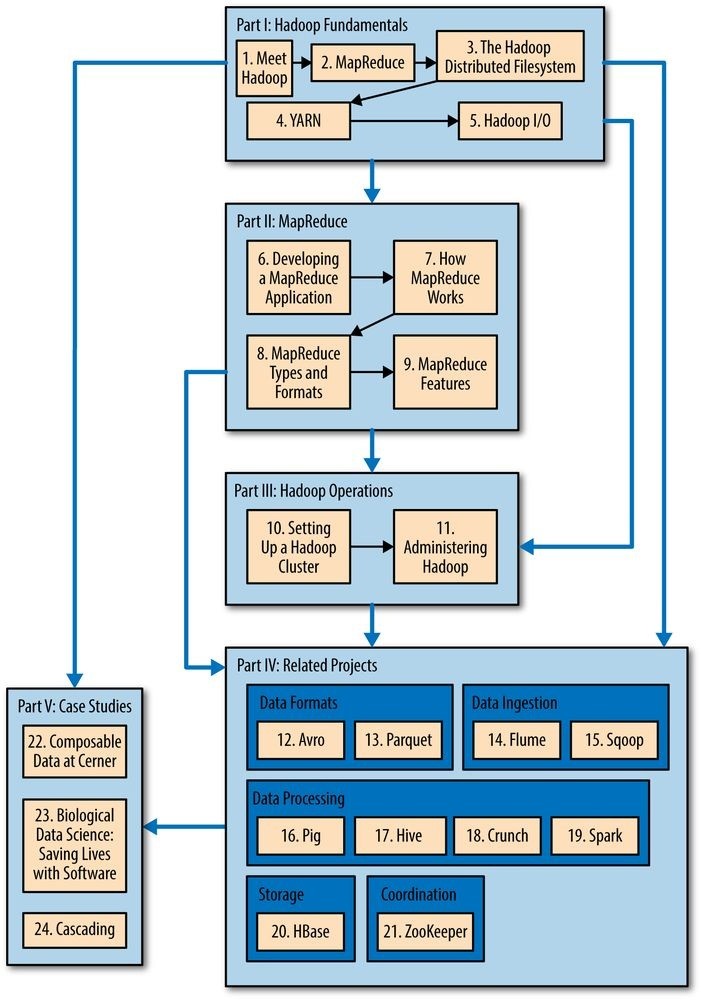
Figure 1-1. Structure of the book: there are various pathways through the content 3[] These statistics were reported in a study entitled “The Digital Universe of Opportunities: Rich Data and the Increasing Value of the Internet of Things.”
[4] All figures are from 2013 or 2014. For more information, see Tom Groenfeldt, “At NYSE, The Data Deluge
Overwhelms Traditional Databases”; Rich Miller, “Facebook Builds Exabyte Data Centers for Cold Storage”; Ancestry.com’s “Company Facts”; Archive.org’s “Petabox”; and the Worldwide LHC Computing Grid project’s welcome page.
[5] The quote is from Anand Rajaraman’s blog post “More data usually beats better algorithms,” in which he writes about the Netflix Challenge. Alon Halevy, Peter Norvig, and Fernando Pereira make the same point in “The Unreasonable Effectiveness of Data,” IEEE Intelligent Systems, March/April 2009.
[6] These specifications are for the Seagate ST-41600n.
[7] In January 2007, David J. DeWitt and Michael Stonebraker caused a stir by publishing “MapReduce: A major step backwards,” in which they criticized MapReduce for being a poor substitute for relational databases. Many commentators argued that it was a false comparison (see, for example, Mark C. Chu-Carroll’s “Databases are hammers; MapReduce is a screwdriver”), and DeWitt and Stonebraker followed up with “MapReduce II,” where they addressed the main topics brought up by others.
[8] Jim Gray was an early advocate of putting the computation near the data. See “Distributed Computing Economics,” March 2003.
[9] In January 2008, SETI@home was reported to be processing 300 gigabytes a day, using 320,000 computers (most of which are not dedicated to SETI@home; they are used for other things, too).
[10] In this book, we use the lowercase form, “namenode,” to denote the entity when it’s being referred to generally, and the CamelCase form NameNode to denote the Java class that implements it.
[11] See Mike Cafarella and Doug Cutting, “Building Nutch: Open Source Search,” ACM Queue, April 2004.
[12] Sanjay Ghemawat, Howard Gobioff, and Shun-Tak Leung, “The Google File System,” October 2003.
[13] Jeffrey Dean and Sanjay Ghemawat, “MapReduce: Simplified Data Processing on Large Clusters,” December 2004.
[14] “Yahoo! Launches World’s Largest Hadoop Production Application,” February 19, 2008.
[15] Derek Gottfrid, “Self-Service, Prorated Super Computing Fun!” November 1, 2007.
[16] Owen O’Malley, “TeraByte Sort on Apache Hadoop,” May 2008.
[17] Grzegorz Czajkowski, “Sorting 1PB with MapReduce,” November 21, 2008.
[18] Owen O’Malley and Arun C. Murthy, “Winning a 60 Second Dash with a Yellow Elephant,” April 2009.
[19] Reynold Xin et al., “GraySort on Apache Spark by Databricks,” November 2014.
Chapter 2. MapReduce
MapReduce is a programming model for data processing. The model is simple, yet not too simple to express useful programs in. Hadoop can run MapReduce programs written in various languages; in this chapter, we look at the same program expressed in Java, Ruby, and Python. Most importantly, MapReduce programs are inherently parallel, thus putting very large-scale data analysis into the hands of anyone with enough machines at their disposal. MapReduce comes into its own for large datasets, so let’s start by looking at one.
A Weather Dataset
For our example, we will write a program that mines weather data. Weather sensors collect data every hour at many locations across the globe and gather a large volume of log data, which is a good candidate for analysis with MapReduce because we want to process all the data, and the data is semi-structured and record-oriented.
Data Format
The data we will use is from the National Climatic Data Center, or NCDC. The data is stored using a line-oriented ASCII format, in which each line is a record. The format supports a rich set of meteorological elements, many of which are optional or with variable data lengths. For simplicity, we focus on the basic elements, such as temperature, which are always present and are of fixed width.
Example 2-1 shows a sample line with some of the salient fields annotated. The line has been split into multiple lines to show each field; in the real file, fields are packed into one line with no delimiters.
Example 2-1. Format of a National Climatic Data Center record
0057
332130 # USAF weather station identifier
99999 # WBAN weather station identifier
19500101 # observation date
0300 # observation time
4
+51317 # latitude (degrees x 1000)
+028783 # longitude (degrees x 1000)
FM-12
+0171 # elevation (meters)
99999
V020
320 # wind direction (degrees)
1 # quality code
N
0072
1
00450 # sky ceiling height (meters)
1 # quality code
C
N
010000 # visibility distance (meters)
1 # quality code
N
9
-0128 # air temperature (degrees Celsius x 10)
1 # quality code
-0139 # dew point temperature (degrees Celsius x 10)
1 # quality code
10268 # atmospheric pressure (hectopascals x 10) 1 # quality code
Datafiles are organized by date and weather station. There is a directory for each year from 1901 to 2001, each containing a gzipped file for each weather station with its readings for that year. For example, here are the first entries for 1990:
% ls raw/1990 | head
010010-99999-1990.gz
010014-99999-1990.gz
010015-99999-1990.gz
010016-99999-1990.gz
010017-99999-1990.gz
010030-99999-1990.gz
010040-99999-1990.gz
010080-99999-1990.gz
010100-99999-1990.gz
010150-99999-1990.gz
There are tens of thousands of weather stations, so the whole dataset is made up of a large number of relatively small files. It’s generally easier and more efficient to process a smaller number of relatively large files, so the data was preprocessed so that each year’s readings were concatenated into a single file. (The means by which this was carried out is described in Appendix C.)
Analyzing the Data with Unix Tools
What’s the highest recorded global temperature for each year in the dataset? We will answer this first without using Hadoop, as this information will provide a performance baseline and a useful means to check our results.
The classic tool for processing line-oriented data is awk. Example 2-2 is a small script to calculate the maximum temperature for each year.
Example 2-2. A program for finding the maximum recorded temperature by year from NCDC weather records
#!/usr/bin/env bash for year in all/ do
echo -ne basename $year .gz“\t” gunzip -c $year | \ awk ‘{ temp = substr($0, 88, 5) + 0; q = substr($0, 93, 1); if (temp !=9999 && q ~ /[01459]/ && temp > max) max = temp } END { print max }’ done
The script loops through the compressed year files, first printing the year, and then processing each file using awk. The awk script extracts two fields from the data: the air temperature and the quality code. The air temperature value is turned into an integer by adding 0. Next, a test is applied to see whether the temperature is valid (the value 9999 signifies a missing value in the NCDC dataset) and whether the quality code indicates that the reading is not suspect or erroneous. If the reading is OK, the value is compared with the maximum value seen so far, which is updated if a new maximum is found. The END block is executed after all the lines in the file have been processed, and it prints the maximum value.
Here is the beginning of a run:
% *./max_temperature.sh
1901 317
1902 244
1903 289
1904 256
1905 283…
The temperature values in the source file are scaled by a factor of 10, so this works out as a maximum temperature of 31.7°C for 1901 (there were very few readings at the beginning of the century, so this is plausible). The complete run for the century took 42 minutes in one run on a single EC2 High-CPU Extra Large instance.
To speed up the processing, we need to run parts of the program in parallel. In theory, this is straightforward: we could process different years in different processes, using all the available hardware threads on a machine. There are a few problems with this, however.
First, dividing the work into equal-size pieces isn’t always easy or obvious. In this case, the file size for different years varies widely, so some processes will finish much earlier than others. Even if they pick up further work, the whole run is dominated by the longest file. A better approach, although one that requires more work, is to split the input into fixed-size chunks and assign each chunk to a process.
Second, combining the results from independent processes may require further processing.
In this case, the result for each year is independent of other years, and they may be combined by concatenating all the results and sorting by year. If using the fixed-size chunk approach, the combination is more delicate. For this example, data for a particular year will typically be split into several chunks, each processed independently. We’ll end up with the maximum temperature for each chunk, so the final step is to look for the highest of these maximums for each year.
Third, you are still limited by the processing capacity of a single machine. If the best time you can achieve is 20 minutes with the number of processors you have, then that’s it. You can’t make it go faster. Also, some datasets grow beyond the capacity of a single machine. When we start using multiple machines, a whole host of other factors come into play, mainly falling into the categories of coordination and reliability. Who runs the overall job? How do we deal with failed processes?
So, although it’s feasible to parallelize the processing, in practice it’s messy. Using a framework like Hadoop to take care of these issues is a great help.
Analyzing the Data with Hadoop
To take advantage of the parallel processing that Hadoop provides, we need to express our query as a MapReduce job. After some local, small-scale testing, we will be able to run it on a cluster of machines.
Map and Reduce
MapReduce works by breaking the processing into two phases: the map phase and the reduce phase. Each phase has key-value pairs as input and output, the types of which may be chosen by the programmer. The programmer also specifies two functions: the map function and the reduce function.
The input to our map phase is the raw NCDC data. We choose a text input format that gives us each line in the dataset as a text value. The key is the offset of the beginning of the line from the beginning of the file, but as we have no need for this, we ignore it.
Our map function is simple. We pull out the year and the air temperature, because these are the only fields we are interested in. In this case, the map function is just a data preparation phase, setting up the data in such a way that the reduce function can do its work on it: finding the maximum temperature for each year. The map function is also a good place to drop bad records: here we filter out temperatures that are missing, suspect, or erroneous.
To visualize the way the map works, consider the following sample lines of input data (some unused columns have been dropped to fit the page, indicated by ellipses):
0067011990999991950051507004…9999999N9+00001+99999999999…
0043011990999991950051512004…9999999N9+00221+99999999999…
0043011990999991950051518004…9999999N9-00111+99999999999…
0043012650999991949032412004…0500001N9+01111+99999999999…
0043012650999991949032418004…0500001N9+00781+99999999999…
These lines are presented to the map function as the key-value pairs:
(0, 0067011990999991950051507004…9999999N9+00001+99999999999…)
(106, 0043011990999991950051512004…9999999N9+00221+99999999999…)
(212, 0043011990999991950051518004…9999999N9-00111+99999999999…)
(318, 0043012650999991949032412004…0500001N9+01111+99999999999…)
(424, 0043012650999991949032418004…0500001N9+00781+99999999999…)
The keys are the line offsets within the file, which we ignore in our map function. The map function merely extracts the year and the air temperature (indicated in bold text), and emits them as its output (the temperature values have been interpreted as integers):
(1950, 0)
(1950, 22)
(1950, −11)
(1949, 111) (1949, 78)
The output from the map function is processed by the MapReduce framework before being sent to the reduce function. This processing sorts and groups the key-value pairs by key. So, continuing the example, our reduce function sees the following input:
(1949, [111, 78])
(1950, [0, 22, −11])
Each year appears with a list of all its air temperature readings. All the reduce function has to do now is iterate through the list and pick up the maximum reading:
(1949, 111) (1950, 22)
This is the final output: the maximum global temperature recorded in each year.
The whole data flow is illustrated in Figure 2-1. At the bottom of the diagram is a Unix pipeline, which mimics the whole MapReduce flow and which we will see again later in this chapter when we look at Hadoop Streaming.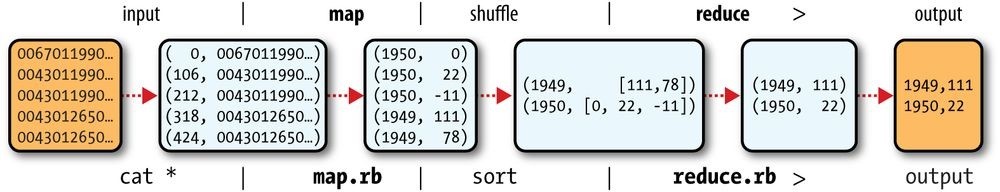
Figure 2-1. MapReduce logical data flow
Java MapReduce
Having run through how the MapReduce program works, the next step is to express it in code. We need three things: a map function, a reduce function, and some code to run the job. The map function is represented by the Mapper class, which declares an abstract map() method. Example 2-3 shows the implementation of our map function. Example 2-3. Mapper for the maximum temperature example
import java.io.IOException;
import org.apache.hadoop.io.IntWritable; import org.apache.hadoop.io.LongWritable; import org.apache.hadoop.io.Text; import org.apache.hadoop.mapreduce.Mapper;
public class MaxTemperatureMapper
extends Mapper
private static final int MISSING = 9999;
@Override
public void map(LongWritable key, Text value, Context context) throws IOException, InterruptedException {
String line = value.toString(); String year = line.substring(15, 19); int airTemperature; if (line.charAt(87) == ‘+’) { // parseInt doesn’t like leading plus signs airTemperature = Integer.parseInt(line.substring(88, 92));
} else {
airTemperature = Integer.parseInt(line.substring(87, 92));
}
String quality = line.substring(92, 93);
if (airTemperature != MISSING && quality.matches(“[01459]”)) { context.write(new Text(year), new IntWritable(airTemperature));
}
} }
The Mapper class is a generic type, with four formal type parameters that specify the input key, input value, output key, and output value types of the map function. For the present example, the input key is a long integer offset, the input value is a line of text, the output key is a year, and the output value is an air temperature (an integer). Rather than using built-in Java types, Hadoop provides its own set of basic types that are optimized for network serialization. These are found in the org.apache.hadoop.io package. Here we use LongWritable, which corresponds to a Java Long, Text (like Java String), and IntWritable (like Java Integer).
The map() method is passed a key and a value. We convert the Text value containing the line of input into a Java String, then use its substring() method to extract the columns we are interested in.
The map() method also provides an instance of Context to write the output to. In this case, we write the year as a Text object (since we are just using it as a key), and the temperature is wrapped in an IntWritable. We write an output record only if the temperature is present and the quality code indicates the temperature reading is OK.
The reduce function is similarly defined using a Reducer, as illustrated in Example 2-4. Example 2-4. Reducer for the maximum temperature example
import java.io.IOException;
import org.apache.hadoop.io.IntWritable; import org.apache.hadoop.io.Text; import org.apache.hadoop.mapreduce.Reducer;
public class MaxTemperatureReducer extends Reducer
@Override
public void reduce(Text key, Iterable
int maxValue = Integer.MIN_VALUE; for (IntWritable value : values) {
maxValue = Math.max(maxValue, value.get());
}
context.write(key, new IntWritable(maxValue));
} }
Again, four formal type parameters are used to specify the input and output types, this time for the reduce function. The input types of the reduce function must match the output types of the map function: Text and IntWritable. And in this case, the output types of the reduce function are Text and IntWritable, for a year and its maximum temperature, which we find by iterating through the temperatures and comparing each with a record of the highest found so far.
The third piece of code runs the MapReduce job (see Example 2-5).
Example 2-5. Application to find the maximum temperature in the weather dataset
import org.apache.hadoop.fs.Path; import org.apache.hadoop.io.IntWritable; import org.apache.hadoop.io.Text; import org.apache.hadoop.mapreduce.Job;
import org.apache.hadoop.mapreduce.lib.input.FileInputFormat; import org.apache.hadoop.mapreduce.lib.output.FileOutputFormat; public class MaxTemperature {
public static void main(String[] args) throws Exception { if (args.length != 2) {
System.err.println(“Usage: MaxTemperature
A test run
After writing a MapReduce job, it’s normal to try it out on a small dataset to flush out any immediate problems with the code. First, install Hadoop in standalone mode (there are instructions for how to do this in Appendix A). This is the mode in which Hadoop runs using the local filesystem with a local job runner. Then, install and compile the examples using the instructions on the book’s website.
Let’s test it on the five-line sample discussed earlier (the output has been slightly reformatted to fit the page, and some lines have been removed):
% export HADOOP_CLASSPATH=hadoop-examples.jar
% hadoop MaxTemperature input/ncdc/sample.txt output
14/09/16 09:48:39 WARN util.NativeCodeLoader: Unable to load native-hadoop library for your platform… using builtin-java classes where applicable
14/09/16 09:48:40 WARN mapreduce.JobSubmitter: Hadoop command-line option parsing not performed. Implement the Tool interface and execute your application with ToolRunner to remedy this.
14/09/16 09:48:40 INFO input.FileInputFormat: Total input paths to process : 1
14/09/16 09:48:40 INFO mapreduce.JobSubmitter: number of splits:1
14/09/16 09:48:40 INFO mapreduce.JobSubmitter: Submitting tokens for job:
joblocal26392882_0001
14/09/16 09:48:40 INFO mapreduce.Job: The url to track the job: http://localhost:8080/
14/09/16 09:48:40 INFO mapreduce.Job: Running job: job_local26392882_0001 14/09/16 09:48:40 INFO mapred.LocalJobRunner: OutputCommitter set in config null
14/09/16 09:48:40 INFO mapred.LocalJobRunner: OutputCommitter is org.apache.hadoop.mapreduce.lib.output.FileOutputCommitter
14/09/16 09:48:40 INFO mapred.LocalJobRunner: Waiting for map tasks
14/09/16 09:48:40 INFO mapred.LocalJobRunner: Starting task: attempt_local26392882_0001_m_000000_0
14/09/16 09:48:40 INFO mapred.Task: Using ResourceCalculatorProcessTree : null
14/09/16 09:48:40 INFO mapred.LocalJobRunner:
14/09/16 09:48:40 INFO mapred.Task: Task:attempt_local26392882_0001_m_000000_0 is done. And is in the process of committing
14/09/16 09:48:40 INFO mapred.LocalJobRunner: map
14/09/16 09:48:40 INFO mapred.Task: Task ‘attempt_local26392882_0001_m_000000_0’ done.
14/09/16 09:48:40 INFO mapred.LocalJobRunner: Finishing task:
attempt_local26392882_0001_m_000000_0
14/09/16 09:48:40 INFO mapred.LocalJobRunner: map task executor complete.
14/09/16 09:48:40 INFO mapred.LocalJobRunner: Waiting for reduce tasks
14/09/16 09:48:40 INFO mapred.LocalJobRunner: Starting task: attempt_local26392882_0001_r_000000_0
14/09/16 09:48:40 INFO mapred.Task: Using ResourceCalculatorProcessTree : null
14/09/16 09:48:40 INFO mapred.LocalJobRunner: 1 / 1 copied.
14/09/16 09:48:40 INFO mapred.Merger: Merging 1 sorted segments
14/09/16 09:48:40 INFO mapred.Merger: Down to the last merge-pass, with 1 segments left of total size: 50 bytes
14/09/16 09:48:40 INFO mapred.Merger: Merging 1 sorted segments
14/09/16 09:48:40 INFO mapred.Merger: Down to the last merge-pass, with 1 segments left of total size: 50 bytes
14/09/16 09:48:40 INFO mapred.LocalJobRunner: 1 / 1 copied.
14/09/16 09:48:40 INFO mapred.Task: Task:attempt_local26392882_0001_r_000000_0 is done. And is in the process of committing
14/09/16 09:48:40 INFO mapred.LocalJobRunner: 1 / 1 copied.
14/09/16 09:48:40 INFO mapred.Task: Task attempt_local26392882_0001_r_000000_0 is allowed to commit now
14/09/16 09:48:40 INFO output.FileOutputCommitter: Saved output of task
‘attempt…local26392882_0001_r_000000_0’ to file:/Users/tom/book-workspace/ hadoop-book/output/_temporary/0/task_local26392882_0001_r_000000
14/09/16 09:48:40 INFO mapred.LocalJobRunner: reduce > reduce
14/09/16 09:48:40 INFO mapred.Task: Task ‘attempt_local26392882_0001_r_000000_0’
done.
14/09/16 09:48:40 INFO mapred.LocalJobRunner: Finishing task:
attempt_local26392882_0001_r_000000_0
14/09/16 09:48:40 INFO mapred.LocalJobRunner: reduce task executor complete.
14/09/16 09:48:41 INFO mapreduce.Job: Job job_local26392882_0001 running in uber mode : false
14/09/16 09:48:41 INFO mapreduce.Job: map 100% reduce 100%
14/09/16 09:48:41 INFO mapreduce.Job: Job job_local26392882_0001 completed successfully
14/09/16 09:48:41 INFO mapreduce.Job: Counters: 30
File System Counters
FILE: Number of bytes read=377168
FILE: Number of bytes written=828464
FILE: Number of read operations=0
FILE: Number of large read operations=0
FILE: Number of write operations=0
Map-Reduce Framework
Map input records=5
Map output records=5
Map output bytes=45
Map output materialized bytes=61
Input split bytes=129
Combine input records=0
Combine output records=0
Reduce input groups=2
Reduce shuffle bytes=61
Reduce input records=5
Reduce output records=2
Spilled Records=10
Shuffled Maps =1
Failed Shuffles=0
Merged Map outputs=1
GC time elapsed (ms)=39
Total committed heap usage (bytes)=226754560
File Input Format Counters
Bytes Read=529
File Output Format Counters
Bytes Written=29
When the hadoop command is invoked with a classname as the first argument, it launches a Java virtual machine (JVM) to run the class. The hadoop command adds the Hadoop libraries (and their dependencies) to the classpath and picks up the Hadoop configuration, too. To add the application classes to the classpath, we’ve defined an environment variable called HADOOP_CLASSPATH, which the _hadoop script picks up.
NOTE
When running in local (standalone) mode, the programs in this book all assume that you have set the HADOOPCLASSPATH in this way. The commands should be run from the directory that the example code is installed in.
The output from running the job provides some useful information. For example, we can see that the job was given an ID of job_local26392882_0001, and it ran one map task and one reduce task (with the following IDs: attempt_local26392882_0001_m_000000_0 and attempt_local26392882_0001_r_000000_0). Knowing the job and task IDs can be very useful when debugging MapReduce jobs.
The last section of the output, titled “Counters,” shows the statistics that Hadoop generates for each job it runs. These are very useful for checking whether the amount of data processed is what you expected. For example, we can follow the number of records that went through the system: five map input records produced five map output records (since the mapper emitted one output record for each valid input record), then five reduce input records in two groups (one for each unique key) produced two reduce output records.
The output was written to the _output directory, which contains one output file per reducer.
The job had a single reducer, so we find a single file, named part-r-00000:
% cat output/part-r-00000
1949 111
1950 22
This result is the same as when we went through it by hand earlier. We interpret this as saying that the maximum temperature recorded in 1949 was 11.1°C, and in 1950 it was 2.2°C.
Scaling Out
You’ve seen how MapReduce works for small inputs; now it’s time to take a bird’s-eye view of the system and look at the data flow for large inputs. For simplicity, the examples so far have used files on the local filesystem. However, to scale out, we need to store the data in a distributed filesystem (typically HDFS, which you’ll learn about in the next chapter). This allows Hadoop to move the MapReduce computation to each machine hosting a part of the data, using Hadoop’s resource management system, called YARN (see Chapter 4). Let’s see how this works.
Data Flow
First, some terminology. A MapReduce job is a unit of work that the client wants to be performed: it consists of the input data, the MapReduce program, and configuration information. Hadoop runs the job by dividing it into tasks, of which there are two types: map tasks and reduce tasks. The tasks are scheduled using YARN and run on nodes in the cluster. If a task fails, it will be automatically rescheduled to run on a different node.
Hadoop divides the input to a MapReduce job into fixed-size pieces called input splits, or just splits. Hadoop creates one map task for each split, which runs the user-defined map function for each record in the split.
Having many splits means the time taken to process each split is small compared to the time to process the whole input. So if we are processing the splits in parallel, the processing is better load balanced when the splits are small, since a faster machine will be able to process proportionally more splits over the course of the job than a slower machine. Even if the machines are identical, failed processes or other jobs running concurrently make load balancing desirable, and the quality of the load balancing increases as the splits become more fine grained.
On the other hand, if splits are too small, the overhead of managing the splits and map task creation begins to dominate the total job execution time. For most jobs, a good split size tends to be the size of an HDFS block, which is 128 MB by default, although this can be changed for the cluster (for all newly created files) or specified when each file is created.
Hadoop does its best to run the map task on a node where the input data resides in HDFS, because it doesn’t use valuable cluster bandwidth. This is called the data locality optimization. Sometimes, however, all the nodes hosting the HDFS block replicas for a map task’s input split are running other map tasks, so the job scheduler will look for a free map slot on a node in the same rack as one of the blocks. Very occasionally even this is not possible, so an off-rack node is used, which results in an inter-rack network transfer. The three possibilities are illustrated in Figure 2-2.
It should now be clear why the optimal split size is the same as the block size: it is the largest size of input that can be guaranteed to be stored on a single node. If the split spanned two blocks, it would be unlikely that any HDFS node stored both blocks, so some of the split would have to be transferred across the network to the node running the map task, which is clearly less efficient than running the whole map task using local data.
Map tasks write their output to the local disk, not to HDFS. Why is this? Map output is intermediate output: it’s processed by reduce tasks to produce the final output, and once the job is complete, the map output can be thrown away. So, storing it in HDFS with replication would be overkill. If the node running the map task fails before the map output has been consumed by the reduce task, then Hadoop will automatically rerun the map task on another node to re-create the map output.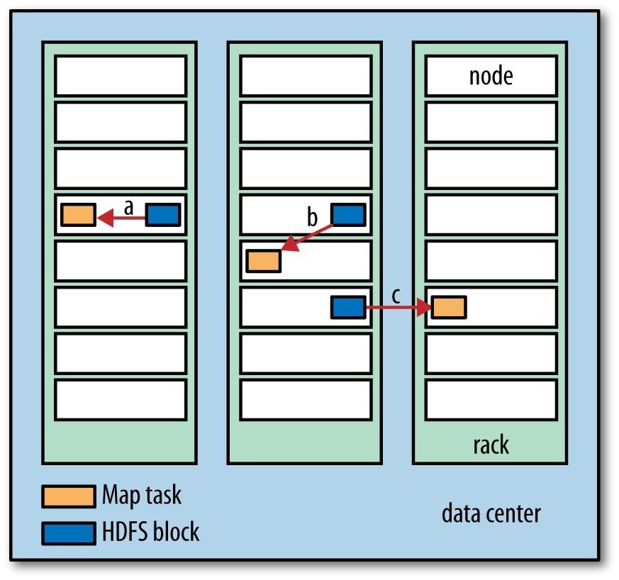
Figure 2-2. Data-local (a), rack-local (b), and off-rack (c) map tasks
Reduce tasks don’t have the advantage of data locality; the input to a single reduce task is normally the output from all mappers. In the present example, we have a single reduce task that is fed by all of the map tasks. Therefore, the sorted map outputs have to be transferred across the network to the node where the reduce task is running, where they are merged and then passed to the user-defined reduce function. The output of the reduce is normally stored in HDFS for reliability. As explained in Chapter 3, for each HDFS block of the reduce output, the first replica is stored on the local node, with other replicas being stored on off-rack nodes for reliability. Thus, writing the reduce output does consume network bandwidth, but only as much as a normal HDFS write pipeline consumes.
The whole data flow with a single reduce task is illustrated in Figure 2-3. The dotted boxes indicate nodes, the dotted arrows show data transfers on a node, and the solid arrows show data transfers between nodes.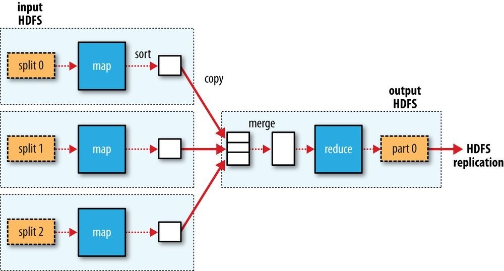
Figure 2-3. MapReduce data flow with a single reduce task
The number of reduce tasks is not governed by the size of the input, but instead is specified independently. In The Default MapReduce Job, you will see how to choose the number of reduce tasks for a given job.
When there are multiple reducers, the map tasks partition their output, each creating one partition for each reduce task. There can be many keys (and their associated values) in each partition, but the records for any given key are all in a single partition. The partitioning can be controlled by a user-defined partitioning function, but normally the default partitioner — which buckets keys using a hash function — works very well.
The data flow for the general case of multiple reduce tasks is illustrated in Figure 2-4. This diagram makes it clear why the data flow between map and reduce tasks is colloquially known as “the shuffle,” as each reduce task is fed by many map tasks. The shuffle is more complicated than this diagram suggests, and tuning it can have a big impact on job execution time, as you will see in Shuffle and Sort.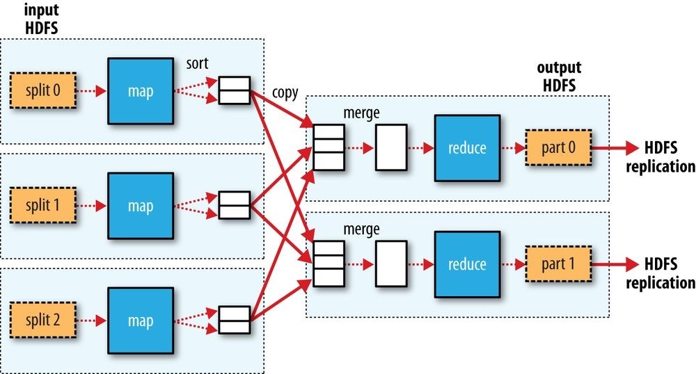
Figure 2-4. MapReduce data flow with multiple reduce tasks
Finally, it’s also possible to have zero reduce tasks. This can be appropriate when you don’t need the shuffle because the processing can be carried out entirely in parallel (a few examples are discussed in NLineInputFormat). In this case, the only off-node data transfer is when the map tasks write to HDFS (see Figure 2-5).
Combiner Functions
Many MapReduce jobs are limited by the bandwidth available on the cluster, so it pays to minimize the data transferred between map and reduce tasks. Hadoop allows the user to specify a combiner function to be run on the map output, and the combiner function’s output forms the input to the reduce function. Because the combiner function is an optimization, Hadoop does not provide a guarantee of how many times it will call it for a particular map output record, if at all. In other words, calling the combiner function zero, one, or many times should produce the same output from the reducer.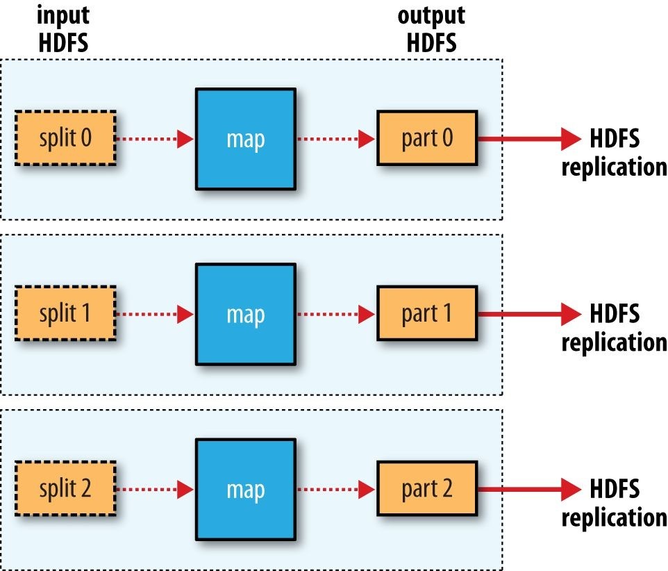
Figure 2-5. MapReduce data flow with no reduce tasks
The contract for the combiner function constrains the type of function that may be used. This is best illustrated with an example. Suppose that for the maximum temperature example, readings for the year 1950 were processed by two maps (because they were in different splits). Imagine the first map produced the output:
(1950, 0)
(1950, 20)
(1950, 10) and the second produced:
(1950, 25)
(1950, 15)
The reduce function would be called with a list of all the values:
(1950, [0, 20, 10, 25, 15]) with output:
(1950, 25) since 25 is the maximum value in the list. We could use a combiner function that, just like the reduce function, finds the maximum temperature for each map output. The reduce function would then be called with:
(1950, [20, 25]) and would produce the same output as before. More succinctly, we may express the function calls on the temperature values in this case as follows: max(0, 20, 10, 25, 15) = max(max(0, 20, 10), max(25, 15)) = max(20, 25) = 25
Not all functions possess this property.20] For example, if we were calculating mean temperatures, we couldn’t use the mean as our combiner function, because: mean(0, 20, 10, 25, 15) = 14
but: mean(mean(0, 20, 10), mean(25, 15)) = mean(10, 20) = 15
The combiner function doesn’t replace the reduce function. (How could it? The reduce function is still needed to process records with the same key from different maps.) But it can help cut down the amount of data shuffled between the mappers and the reducers, and for this reason alone it is always worth considering whether you can use a combiner function in your MapReduce job. Specifying a combiner function
Going back to the Java MapReduce program, the combiner function is defined using the Reducer class, and for this application, it is the same implementation as the reduce function in MaxTemperatureReducer. The only change we need to make is to set the combiner class on the Job (see Example 2-6).
Example 2-6. Application to find the maximum temperature, using a combiner function for efficiency
public class MaxTemperatureWithCombiner {
public static void main(String[] args) throws Exception { if (args.length != 2) {
System.err.println(“Usage: MaxTemperatureWithCombiner “ +
“
Running a Distributed MapReduce Job
The same program will run, without alteration, on a full dataset. This is the point of MapReduce: it scales to the size of your data and the size of your hardware. Here’s one data point: on a 10-node EC2 cluster running High-CPU Extra Large instances, the program took six minutes to run.21]
We’ll go through the mechanics of running programs on a cluster in Chapter 6.
Hadoop Streaming
Hadoop provides an API to MapReduce that allows you to write your map and reduce functions in languages other than Java. Hadoop Streaming uses Unix standard streams as the interface between Hadoop and your program, so you can use any language that can read standard input and write to standard output to write your MapReduce program.22]
Streaming is naturally suited for text processing. Map input data is passed over standard input to your map function, which processes it line by line and writes lines to standard output. A map output key-value pair is written as a single tab-delimited line. Input to the reduce function is in the same format — a tab-separated key-value pair — passed over standard input. The reduce function reads lines from standard input, which the framework guarantees are sorted by key, and writes its results to standard output.
Let’s illustrate this by rewriting our MapReduce program for finding maximum temperatures by year in Streaming.
Ruby
The map function can be expressed in Ruby as shown in Example 2-7.
Example 2-7. Map function for maximum temperature in Ruby
#!/usr/bin/env ruby
STDIN.each_line do |line| val = line year, temp, q = val[15,4], val[87,5], val[92,1] puts “#{year}\t#{temp}” if (temp != “+9999” && q =~ /[01459]/) end
The program iterates over lines from standard input by executing a block for each line from STDIN (a global constant of type IO). The block pulls out the relevant fields from each input line and, if the temperature is valid, writes the year and the temperature separated by a tab character, \t, to standard output (using puts).
NOTE It’s worth drawing out a design difference between Streaming and the Java MapReduce API. The Java API is geared toward processing your map function one record at a time. The framework calls the map() method on your Mapper for each record in the input, whereas with Streaming the map program can decide how to process the input — for example, it could easily read and process multiple lines at a time since it’s in control of the reading. The user’s Java map implementation is “pushed” records, but it’s still possible to consider multiple lines at a time by accumulating previous lines in an instance variable in the Mapper.[23] In this case, you need to implement the close() method so that you know when the last record has been read, so you can finish processing the last group of lines.
Because the script just operates on standard input and output, it’s trivial to test the script without using Hadoop, simply by using Unix pipes:
% cat input/ncdc/sample.txt | ch02-mr-intro/src/main/ruby/max_temperature_map.rb
1950 +0000
1950 +0022
1950 -0011
1949 +0111
1949 +0078
The reduce function shown in Example 2-8 is a little more complex.
Example 2-8. Reduce function for maximum temperature in Ruby
#!/usr/bin/env ruby
last_key, max_val = nil, -1000000
STDIN.each_line do |line| key, val = line.split(“\t“) if last_key && last_key != key puts “#{last_key}\t#{max_val}” last_key, max_val = key, val.to_i else
last_key, max_val = key, [max_val, val.to_i].max end end puts “#{last_key}\t#{max_val}” if last_key
Again, the program iterates over lines from standard input, but this time we have to store some state as we process each key group. In this case, the keys are the years, and we store the last key seen and the maximum temperature seen so far for that key. The MapReduce framework ensures that the keys are ordered, so we know that if a key is different from the previous one, we have moved into a new key group. In contrast to the Java API, where you are provided an iterator over each key group, in Streaming you have to find key group boundaries in your program.
For each line, we pull out the key and value. Then, if we’ve just finished a group
(last_key && last_key != key), we write the key and the maximum temperature for that group, separated by a tab character, before resetting the maximum temperature for the new key. If we haven’t just finished a group, we just update the maximum temperature for the current key.
The last line of the program ensures that a line is written for the last key group in the input.
We can now simulate the whole MapReduce pipeline with a Unix pipeline (which is equivalent to the Unix pipeline shown in Figure 2-1):
% cat input/ncdc/sample.txt | \
ch02-mr-intro/src/main/ruby/max_temperature_map.rb | \ sort | ch02-mr-intro/src/main/ruby/max_temperature_reduce.rb
1949 111
1950 22
The output is the same as that of the Java program, so the next step is to run it using Hadoop itself.
The hadoop command doesn’t support a Streaming option; instead, you specify the Streaming JAR file along with the jar option. Options to the Streaming program specify the input and output paths and the map and reduce scripts. This is what it looks like:
% hadoop jar $HADOOP_HOME/share/hadoop/tools/lib/hadoop-streaming-*.jar \
-input input/ncdc/sample.txt \
-output output \
-mapper ch02-mr-intro/src/main/ruby/max_temperature_map.rb \
-reducer ch02-mr-intro/src/main/ruby/max_temperature_reduce.rb
When running on a large dataset on a cluster, we should use the -combiner option to set the combiner:
% hadoop jar $HADOOP_HOME/share/hadoop/tools/lib/hadoop-streaming-*.jar \
-files ch02-mr-intro/src/main/ruby/max_temperature_map.rb,\ ch02-mr-intro/src/main/ruby/max_temperature_reduce.rb \
-input input/ncdc/all \
-output output \
-mapper ch02-mr-intro/src/main/ruby/max_temperature_map.rb \
-combiner ch02-mr-intro/src/main/ruby/max_temperature_reduce.rb \
-reducer ch02-mr-intro/src/main/ruby/max_temperature_reduce.rb
Note also the use of -files, which we use when running Streaming programs on the cluster to ship the scripts to the cluster.
Python
Streaming supports any programming language that can read from standard input and write to standard output, so for readers more familiar with Python, here’s the same example again.24] The map script is in Example 2-9, and the reduce script is in Example 2-10.
Example 2-9. Map function for maximum temperature in Python
#!/usr/bin/env python
import re import sys
for line in sys.stdin: val = line.strip()
(year, temp, q) = (val[15:19], val[87:92], val[92:93]) if (temp != “+9999” and re.match(“[01459]”, q)): print “%s\t%s” % (year, temp)
Example 2-10. Reduce function for maximum temperature in Python
#!/usr/bin/env python import sys
(lastkey, max_val) = (None, -sys.maxint) for line in sys.stdin:
(key, val) = line.strip().split(“\t“) if last_key and last_key != key:
print “%s\t%s” % (last_key, max_val) (last_key, max_val) = (key, int(val)) else:
(last_key, max_val) = (key, max(max_val, int(val)))
if last_key: print “%s\t%s” % (last_key, max_val)
We can test the programs and run the job in the same way we did in Ruby. For example, to run a test:
% cat input/ncdc/sample.txt | \
ch02-mr-intro/src/main/python/max_temperature_map.py | \ sort | ch02-mr-intro/src/main/python/max_temperature_reduce.py
1949 111
1950 22
[20] Functions with this property are called _commutative and associative. They are also sometimes referred to as distributive, such as by Jim Gray et al.’s “Data Cube: A Relational Aggregation Operator Generalizing Group-By, CrossTab, and Sub-Totals,” February1995.
[21] This is a factor of seven faster than the serial run on one machine using awk. The main reason it wasn’t proportionately faster is because the input data wasn’t evenly partitioned. For convenience, the input files were gzipped by year, resulting in large files for later years in the dataset, when the number of weather records was much higher.
[22] Hadoop Pipes is an alternative to Streaming for C++ programmers. It uses sockets to communicate with the process running the C++ map or reduce function.
[23] Alternatively, you could use “pull”-style processing in the new MapReduce API; see Appendix D.
[24] As an alternative to Streaming, Python programmers should consider Dumbo, which makes the Streaming MapReduce interface more Pythonic and easier to use.
Chapter 3. The Hadoop Distributed Filesystem
When a dataset outgrows the storage capacity of a single physical machine, it becomes necessary to partition it across a number of separate machines. Filesystems that manage the storage across a network of machines are called distributed filesystems. Since they are network based, all the complications of network programming kick in, thus making distributed filesystems more complex than regular disk filesystems. For example, one of the biggest challenges is making the filesystem tolerate node failure without suffering data loss.
Hadoop comes with a distributed filesystem called HDFS, which stands for Hadoop Distributed Filesystem. (You may sometimes see references to “DFS” — informally or in older documentation or configurations — which is the same thing.) HDFS is Hadoop’s flagship filesystem and is the focus of this chapter, but Hadoop actually has a generalpurpose filesystem abstraction, so we’ll see along the way how Hadoop integrates with other storage systems (such as the local filesystem and Amazon S3).
The Design of HDFS
HDFS is a filesystem designed for storing very large files with streaming data access patterns, running on clusters of commodity hardware.25] Let’s examine this statement in more detail:
Very large files
“Very large” in this context means files that are hundreds of megabytes, gigabytes, or terabytes in size. There are Hadoop clusters running today that store petabytes of data.
[26]
Streaming data access
HDFS is built around the idea that the most efficient data processing pattern is a writeonce, read-many-times pattern. A dataset is typically generated or copied from source, and then various analyses are performed on that dataset over time. Each analysis will involve a large proportion, if not all, of the dataset, so the time to read the whole dataset is more important than the latency in reading the first record.
Commodity hardware
Hadoop doesn’t require expensive, highly reliable hardware. It’s designed to run on clusters of commodity hardware (commonly available hardware that can be obtained from multiple vendors)27] for which the chance of node failure across the cluster is high, at least for large clusters. HDFS is designed to carry on working without a noticeable interruption to the user in the face of such failure.
It is also worth examining the applications for which using HDFS does not work so well. Although this may change in the future, these are areas where HDFS is not a good fit today:
Low-latency data access
Applications that require low-latency access to data, in the tens of milliseconds range, will not work well with HDFS. Remember, HDFS is optimized for delivering a high throughput of data, and this may be at the expense of latency. HBase (see Chapter 20) is currently a better choice for low-latency access.
Lots of small files
Because the namenode holds filesystem metadata in memory, the limit to the number of files in a filesystem is governed by the amount of memory on the namenode. As a rule of thumb, each file, directory, and block takes about 150 bytes. So, for example, if you had one million files, each taking one block, you would need at least 300 MB of memory. Although storing millions of files is feasible, billions is beyond the capability of current hardware.28]
Multiple writers, arbitrary file modifications
Files in HDFS may be written to by a single writer. Writes are always made at the end of the file, in append-only fashion. There is no support for multiple writers or for modifications at arbitrary offsets in the file. (These might be supported in the future, but they are likely to be relatively inefficient.)
HDFS Concepts
Blocks
A disk has a block size, which is the minimum amount of data that it can read or write. Filesystems for a single disk build on this by dealing with data in blocks, which are an integral multiple of the disk block size. Filesystem blocks are typically a few kilobytes in size, whereas disk blocks are normally 512 bytes. This is generally transparent to the filesystem user who is simply reading or writing a file of whatever length. However, there are tools to perform filesystem maintenance, such as df and fsck, that operate on the filesystem block level.
HDFS, too, has the concept of a block, but it is a much larger unit — 128 MB by default. Like in a filesystem for a single disk, files in HDFS are broken into block-sized chunks, which are stored as independent units. Unlike a filesystem for a single disk, a file in HDFS that is smaller than a single block does not occupy a full block’s worth of underlying storage. (For example, a 1 MB file stored with a block size of 128 MB uses 1 MB of disk space, not 128 MB.) When unqualified, the term “block” in this book refers to a block in
HDFS.
WHY IS A BLOCK IN HDFS SO LARGE?
HDFS blocks are large compared to disk blocks, and the reason is to minimize the cost of seeks. If the block is large enough, the time it takes to transfer the data from the disk can be significantly longer than the time to seek to the start of the block. Thus, transferring a large file made of multiple blocks operates at the disk transfer rate. A quick calculation shows that if the seek time is around 10 ms and the transfer rate is 100 MB/s, to make the seek time 1% of the transfer time, we need to make the block size around 100 MB. The default is actually 128 MB, although many HDFS installations use larger block sizes. This figure will continue to be revised upward as transfer speeds grow with new generations of disk drives.
This argument shouldn’t be taken too far, however. Map tasks in MapReduce normally operate on one block at a time, so if you have too few tasks (fewer than nodes in the cluster), your jobs will run slower than they could otherwise.
Having a block abstraction for a distributed filesystem brings several benefits. The first benefit is the most obvious: a file can be larger than any single disk in the network. There’s nothing that requires the blocks from a file to be stored on the same disk, so they can take advantage of any of the disks in the cluster. In fact, it would be possible, if unusual, to store a single file on an HDFS cluster whose blocks filled all the disks in the cluster.
Second, making the unit of abstraction a block rather than a file simplifies the storage subsystem. Simplicity is something to strive for in all systems, but it is especially important for a distributed system in which the failure modes are so varied. The storage subsystem deals with blocks, simplifying storage management (because blocks are a fixed size, it is easy to calculate how many can be stored on a given disk) and eliminating metadata concerns (because blocks are just chunks of data to be stored, file metadata such as permissions information does not need to be stored with the blocks, so another system can handle metadata separately).
Furthermore, blocks fit well with replication for providing fault tolerance and availability. To insure against corrupted blocks and disk and machine failure, each block is replicated to a small number of physically separate machines (typically three). If a block becomes unavailable, a copy can be read from another location in a way that is transparent to the client. A block that is no longer available due to corruption or machine failure can be replicated from its alternative locations to other live machines to bring the replication factor back to the normal level. (See Data Integrity for more on guarding against corrupt data.) Similarly, some applications may choose to set a high replication factor for the blocks in a popular file to spread the read load on the cluster.
Like its disk filesystem cousin, HDFS’s fsck command understands blocks. For example, running:
% hdfs fsck / -files -blocks will list the blocks that make up each file in the filesystem. (See also Filesystem check (fsck).)
Namenodes and Datanodes
An HDFS cluster has two types of nodes operating in a master−worker pattern: a namenode (the master) and a number of datanodes (workers). The namenode manages the filesystem namespace. It maintains the filesystem tree and the metadata for all the files and directories in the tree. This information is stored persistently on the local disk in the form of two files: the namespace image and the edit log. The namenode also knows the datanodes on which all the blocks for a given file are located; however, it does not store block locations persistently, because this information is reconstructed from datanodes when the system starts.
A client accesses the filesystem on behalf of the user by communicating with the namenode and datanodes. The client presents a filesystem interface similar to a Portable Operating System Interface (POSIX), so the user code does not need to know about the namenode and datanodes to function.
Datanodes are the workhorses of the filesystem. They store and retrieve blocks when they are told to (by clients or the namenode), and they report back to the namenode periodically with lists of blocks that they are storing.
Without the namenode, the filesystem cannot be used. In fact, if the machine running the namenode were obliterated, all the files on the filesystem would be lost since there would be no way of knowing how to reconstruct the files from the blocks on the datanodes. For this reason, it is important to make the namenode resilient to failure, and Hadoop provides two mechanisms for this.
The first way is to back up the files that make up the persistent state of the filesystem metadata. Hadoop can be configured so that the namenode writes its persistent state to multiple filesystems. These writes are synchronous and atomic. The usual configuration choice is to write to local disk as well as a remote NFS mount.
It is also possible to run a secondary namenode, which despite its name does not act as a namenode. Its main role is to periodically merge the namespace image with the edit log to prevent the edit log from becoming too large. The secondary namenode usually runs on a separate physical machine because it requires plenty of CPU and as much memory as the namenode to perform the merge. It keeps a copy of the merged namespace image, which can be used in the event of the namenode failing. However, the state of the secondary namenode lags that of the primary, so in the event of total failure of the primary, data loss is almost certain. The usual course of action in this case is to copy the namenode’s metadata files that are on NFS to the secondary and run it as the new primary. (Note that it is possible to run a hot standby namenode instead of a secondary, as discussed in HDFS High Availability.)
See The filesystem image and edit log for more details.
Block Caching
Normally a datanode reads blocks from disk, but for frequently accessed files the blocks may be explicitly cached in the datanode’s memory, in an off-heap block cache. By default, a block is cached in only one datanode’s memory, although the number is configurable on a per-file basis. Job schedulers (for MapReduce, Spark, and other frameworks) can take advantage of cached blocks by running tasks on the datanode where a block is cached, for increased read performance. A small lookup table used in a join is a good candidate for caching, for example.
Users or applications instruct the namenode which files to cache (and for how long) by adding a cache directive to a cache pool. Cache pools are an administrative grouping for managing cache permissions and resource usage.
HDFS Federation
The namenode keeps a reference to every file and block in the filesystem in memory, which means that on very large clusters with many files, memory becomes the limiting factor for scaling (see How Much Memory Does a Namenode Need?). HDFS federation, introduced in the 2.x release series, allows a cluster to scale by adding namenodes, each of which manages a portion of the filesystem namespace. For example, one namenode might manage all the files rooted under /user, say, and a second namenode might handle files under /share.
Under federation, each namenode manages a namespace volume, which is made up of the metadata for the namespace, and a block pool containing all the blocks for the files in the namespace. Namespace volumes are independent of each other, which means namenodes do not communicate with one another, and furthermore the failure of one namenode does not affect the availability of the namespaces managed by other namenodes. Block pool storage is not partitioned, however, so datanodes register with each namenode in the cluster and store blocks from multiple block pools.
To access a federated HDFS cluster, clients use client-side mount tables to map file paths to namenodes. This is managed in configuration using ViewFileSystem and the viewfs:// URIs.
HDFS High Availability
The combination of replicating namenode metadata on multiple filesystems and using the secondary namenode to create checkpoints protects against data loss, but it does not provide high availability of the filesystem. The namenode is still a single point of failure (SPOF). If it did fail, all clients — including MapReduce jobs — would be unable to read, write, or list files, because the namenode is the sole repository of the metadata and the file-to-block mapping. In such an event, the whole Hadoop system would effectively be out of service until a new namenode could be brought online.
To recover from a failed namenode in this situation, an administrator starts a new primary namenode with one of the filesystem metadata replicas and configures datanodes and clients to use this new namenode. The new namenode is not able to serve requests until it has (i) loaded its namespace image into memory, (ii) replayed its edit log, and (iii) received enough block reports from the datanodes to leave safe mode. On large clusters with many files and blocks, the time it takes for a namenode to start from cold can be 30 minutes or more.
The long recovery time is a problem for routine maintenance, too. In fact, because unexpected failure of the namenode is so rare, the case for planned downtime is actually more important in practice.
Hadoop 2 remedied this situation by adding support for HDFS high availability (HA). In this implementation, there are a pair of namenodes in an active-standby configuration. In the event of the failure of the active namenode, the standby takes over its duties to continue servicing client requests without a significant interruption. A few architectural changes are needed to allow this to happen: The namenodes must use highly available shared storage to share the edit log. When a standby namenode comes up, it reads up to the end of the shared edit log to synchronize its state with the active namenode, and then continues to read new entries as they are written by the active namenode.
 Datanodes must send block reports to both namenodes because the block mappings are stored in a namenode’s memory, and not on disk.
Clients must be configured to handle namenode failover, using a mechanism that is transparent to users.
The secondary namenode’s role is subsumed by the standby, which takes periodic checkpoints of the active namenode’s namespace.
There are two choices for the highly available shared storage: an NFS filer, or a quorum journal manager (QJM). The QJM is a dedicated HDFS implementation, designed for the sole purpose of providing a highly available edit log, and is the recommended choice for most HDFS installations. The QJM runs as a group of journal nodes, and each edit must be written to a majority of the journal nodes. Typically, there are three journal nodes, so the system can tolerate the loss of one of them. This arrangement is similar to the way ZooKeeper works, although it is important to realize that the QJM implementation does not use ZooKeeper. (Note, however, that HDFS HA does use ZooKeeper for electing the active namenode, as explained in the next section.)
If the active namenode fails, the standby can take over very quickly (in a few tens of seconds) because it has the latest state available in memory: both the latest edit log entries and an up-to-date block mapping. The actual observed failover time will be longer in practice (around a minute or so), because the system needs to be conservative in deciding that the active namenode has failed.
In the unlikely event of the standby being down when the active fails, the administrator can still start the standby from cold. This is no worse than the non-HA case, and from an operational point of view it’s an improvement, because the process is a standard operational procedure built into Hadoop.
Failover and fencing
The transition from the active namenode to the standby is managed by a new entity in the system called the failover controller. There are various failover controllers, but the default implementation uses ZooKeeper to ensure that only one namenode is active. Each namenode runs a lightweight failover controller process whose job it is to monitor its namenode for failures (using a simple heartbeating mechanism) and trigger a failover should a namenode fail.
Failover may also be initiated manually by an administrator, for example, in the case of routine maintenance. This is known as a graceful failover, since the failover controller arranges an orderly transition for both namenodes to switch roles.
In the case of an ungraceful failover, however, it is impossible to be sure that the failed namenode has stopped running. For example, a slow network or a network partition can trigger a failover transition, even though the previously active namenode is still running and thinks it is still the active namenode. The HA implementation goes to great lengths to ensure that the previously active namenode is prevented from doing any damage and causing corruption — a method known as fencing.
The QJM only allows one namenode to write to the edit log at one time; however, it is still possible for the previously active namenode to serve stale read requests to clients, so setting up an SSH fencing command that will kill the namenode’s process is a good idea. Stronger fencing methods are required when using an NFS filer for the shared edit log, since it is not possible to only allow one namenode to write at a time (this is why QJM is recommended). The range of fencing mechanisms includes revoking the namenode’s access to the shared storage directory (typically by using a vendor-specific NFS command), and disabling its network port via a remote management command. As a last resort, the previously active namenode can be fenced with a technique rather graphically known as STONITH, or “shoot the other node in the head,” which uses a specialized power distribution unit to forcibly power down the host machine.
Client failover is handled transparently by the client library. The simplest implementation uses client-side configuration to control failover. The HDFS URI uses a logical hostname that is mapped to a pair of namenode addresses (in the configuration file), and the client library tries each namenode address until the operation succeeds.
The Command-Line Interface
We’re going to have a look at HDFS by interacting with it from the command line. There are many other interfaces to HDFS, but the command line is one of the simplest and, to many developers, the most familiar.
We are going to run HDFS on one machine, so first follow the instructions for setting up Hadoop in pseudodistributed mode in Appendix A. Later we’ll see how to run HDFS on a cluster of machines to give us scalability and fault tolerance.
There are two properties that we set in the pseudodistributed configuration that deserve further explanation. The first is fs.defaultFS, set to hdfs://localhost/, which is used to set a default filesystem for Hadoop.29] Filesystems are specified by a URI, and here we have used an hdfs URI to configure Hadoop to use HDFS by default. The HDFS daemons will use this property to determine the host and port for the HDFS namenode. We’ll be running it on localhost, on the default HDFS port, 8020. And HDFS clients will use this property to work out where the namenode is running so they can connect to it.
We set the second property, dfs.replication, to 1 so that HDFS doesn’t replicate filesystem blocks by the default factor of three. When running with a single datanode, HDFS can’t replicate blocks to three datanodes, so it would perpetually warn about blocks being under-replicated. This setting solves that problem.
Basic Filesystem Operations
The filesystem is ready to be used, and we can do all of the usual filesystem operations, such as reading files, creating directories, moving files, deleting data, and listing directories. You can type hadoop fs -help to get detailed help on every command.
Start by copying a file from the local filesystem to HDFS:
% hadoop fs -copyFromLocal input/docs/quangle.txt \ hdfs://localhost/user/tom/quangle.txt
This command invokes Hadoop’s filesystem shell command fs, which supports a number of subcommands — in this case, we are running -copyFromLocal. The local file quangle.txt is copied to the file /user/tom/quangle.txt on the HDFS instance running on localhost. In fact, we could have omitted the scheme and host of the URI and picked up the default, hdfs://localhost, as specified in core-site.xml:
% hadoop fs -copyFromLocal input/docs/quangle.txt /user/tom/quangle.txt
We also could have used a relative path and copied the file to our home directory in HDFS, which in this case is /user/tom:
% hadoop fs -copyFromLocal input/docs/quangle.txt quangle.txt
Let’s copy the file back to the local filesystem and check whether it’s the same:
% hadoop fs -copyToLocal quangle.txt quangle.copy.txt
% md5 input/docs/quangle.txt quangle.copy.txt
MD5 (input/docs/quangle.txt) = e7891a2627cf263a079fb0f18256ffb2
MD5 (quangle.copy.txt) = e7891a2627cf263a079fb0f18256ffb2
The MD5 digests are the same, showing that the file survived its trip to HDFS and is back intact.
Finally, let’s look at an HDFS file listing. We create a directory first just to see how it is displayed in the listing:
% hadoop fs -mkdir books
% hadoop fs -ls . Found 2 items
drwxr-xr-x - tom supergroup 0 2014-10-04 13:22 books -rw-r—r— 1 tom supergroup 119 2014-10-04 13:21 quangle.txt
The information returned is very similar to that returned by the Unix command ls -l, with a few minor differences. The first column shows the file mode. The second column is the replication factor of the file (something a traditional Unix filesystem does not have). Remember we set the default replication factor in the site-wide configuration to be 1, which is why we see the same value here. The entry in this column is empty for directories because the concept of replication does not apply to them — directories are treated as metadata and stored by the namenode, not the datanodes. The third and fourth columns show the file owner and group. The fifth column is the size of the file in bytes, or zero for directories. The sixth and seventh columns are the last modified date and time. Finally, the eighth column is the name of the file or directory.
FILE PERMISSIONS IN HDFS
HDFS has a permissions model for files and directories that is much like the POSIX model. There are three types of permission: the read permission (r), the write permission (w), and the execute permission (x). The read permission is required to read files or list the contents of a directory. The write permission is required to write a file or, for a directory, to create or delete files or directories in it. The execute permission is ignored for a file because you can’t execute a file on HDFS (unlike POSIX), and for a directory this permission is required to access its children.
Each file and directory has an owner, a group, and a mode. The mode is made up of the permissions for the user who is the owner, the permissions for the users who are members of the group, and the permissions for users who are neither the owners nor members of the group. By default, Hadoop runs with security disabled, which means that a client’s identity is not authenticated. Because clients are remote, it is possible for a client to become an arbitrary user simply by creating an account of that name on the remote system. This is not possible if security is turned on; see Security. Either way, it is worthwhile having permissions enabled (as they are by default; see the dfs.permissions.enabled property) to avoid accidental modification or deletion of substantial parts of the filesystem, either by users or by automated tools or programs.
When permissions checking is enabled, the owner permissions are checked if the client’s username matches the owner, and the group permissions are checked if the client is a member of the group; otherwise, the other permissions are checked.
There is a concept of a superuser, which is the identity of the namenode process. Permissions checks are not performed for the superuser.
Hadoop Filesystems
Hadoop has an abstract notion of filesystems, of which HDFS is just one implementation.
The Java abstract class org.apache.hadoop.fs.FileSystem represents the client interface to a filesystem in Hadoop, and there are several concrete implementations. The main ones that ship with Hadoop are described in Table 3-1.
Table 3-1. Hadoop filesystems
Filesystem URI Java implementation (all under org.apache.hadoop) Description scheme
| Local | file | fs.LocalFileSystem | A filesystem for a locally connected disk with client-side checksums. Use RawLocalFileSystem for a local filesystem with no checksums. See LocalFileSystem. |
|---|---|---|---|
| HDFS | hdfs | hdfs.DistributedFileSystem | Hadoop’s distributed filesystem. HDFS is designed to work efficiently in conjunction with MapReduce. |
| WebHDFS | webhdfs | hdfs.web.WebHdfsFileSystem | A filesystem providing authenticated read/write access to HDFS over HTTP. See HTTP. |
| Secure WebHDFS |
swebhdfs | hdfs.web.SWebHdfsFileSystem | The HTTPS version of WebHDFS. |
HAR har fs.HarFileSystem A filesystem layered on another
filesystem for archiving files. Hadoop Archives are used for packing lots of files in HDFS into a single archive file to reduce the namenode’s memory usage. Use the hadoop archive command to create HAR files.
| View | viewfs | viewfs.ViewFileSystem | A client-side mount table for other Hadoop filesystems. Commonly used to create mount points for federated namenodes (see HDFS Federation). |
|---|---|---|---|
| FTP | ftp | fs.ftp.FTPFileSystem | A filesystem backed by an FTP server. |
| S3 | s3a | fs.s3a.S3AFileSystem | A filesystem backed by Amazon S3. Replaces the older s3n (S3 native) implementation. |
| Azure | wasb | fs.azure.NativeAzureFileSystem | A filesystem backed by Microsoft Azure. |
| Swift | swift | fs.swift.snative.SwiftNativeFileSystem | A filesystem backed by OpenStack Swift. |
Hadoop provides many interfaces to its filesystems, and it generally uses the URI scheme to pick the correct filesystem instance to communicate with. For example, the filesystem shell that we met in the previous section operates with all Hadoop filesystems. To list the files in the root directory of the local filesystem, type:
% hadoop fs -ls file:///
Although it is possible (and sometimes very convenient) to run MapReduce programs that access any of these filesystems, when you are processing large volumes of data you should choose a distributed filesystem that has the data locality optimization, notably HDFS (see Scaling Out).
Interfaces
Hadoop is written in Java, so most Hadoop filesystem interactions are mediated through the Java API. The filesystem shell, for example, is a Java application that uses the Java FileSystem class to provide filesystem operations. The other filesystem interfaces are discussed briefly in this section. These interfaces are most commonly used with HDFS, since the other filesystems in Hadoop typically have existing tools to access the underlying filesystem (FTP clients for FTP, S3 tools for S3, etc.), but many of them will work with any Hadoop filesystem.
HTTP
By exposing its filesystem interface as a Java API, Hadoop makes it awkward for nonJava applications to access HDFS. The HTTP REST API exposed by the WebHDFS protocol makes it easier for other languages to interact with HDFS. Note that the HTTP interface is slower than the native Java client, so should be avoided for very large data transfers if possible.
There are two ways of accessing HDFS over HTTP: directly, where the HDFS daemons serve HTTP requests to clients; and via a proxy (or proxies), which accesses HDFS on the client’s behalf using the usual DistributedFileSystem API. The two ways are illustrated in Figure 3-1. Both use the WebHDFS protocol.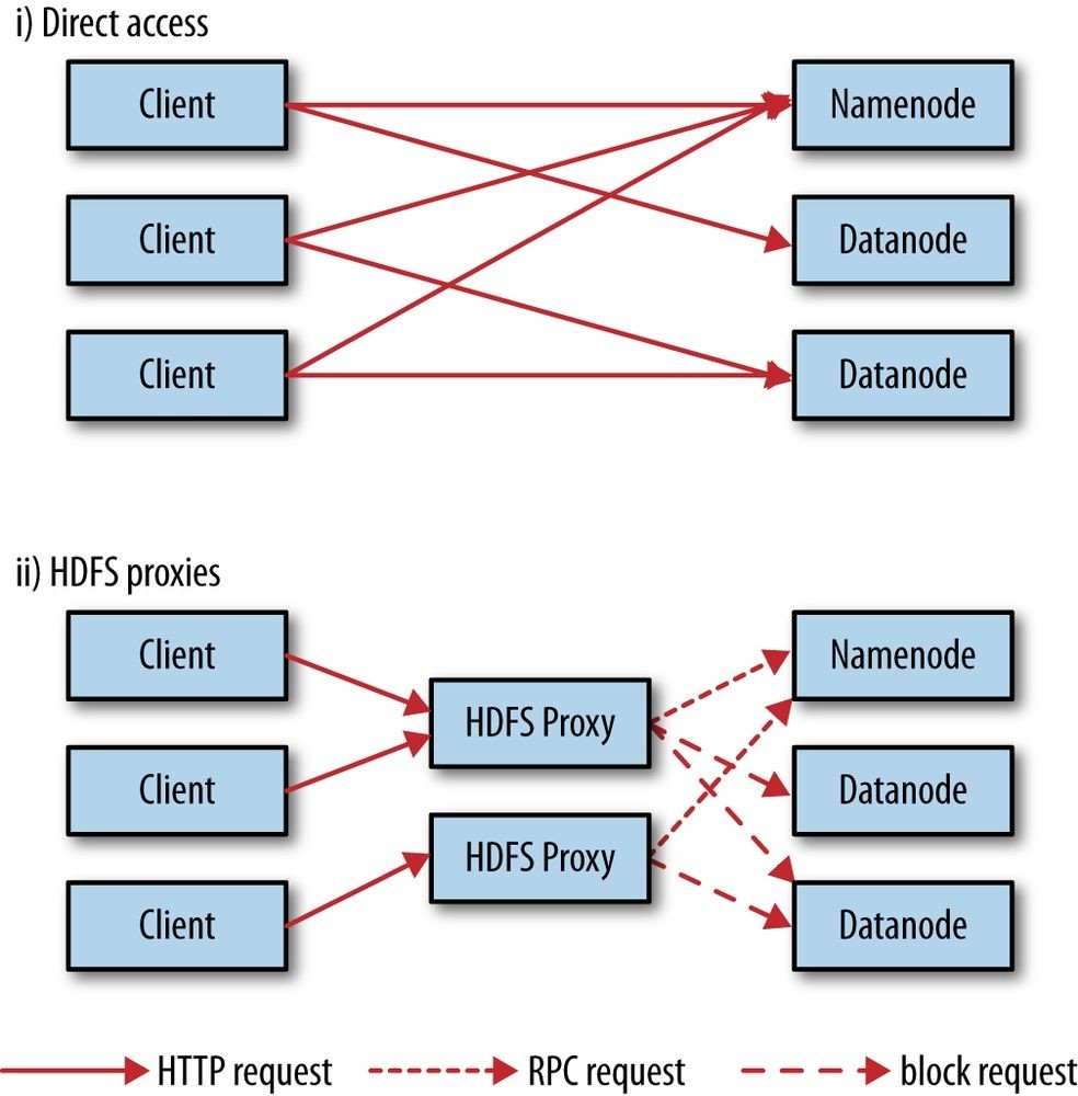
Figure 3-1. Accessing HDFS over HTTP directly and via a bank of HDFS proxies
In the first case, the embedded web servers in the namenode and datanodes act as
WebHDFS endpoints. (WebHDFS is enabled by default, since dfs.webhdfs.enabled is set to true.) File metadata operations are handled by the namenode, while file read (and write) operations are sent first to the namenode, which sends an HTTP redirect to the client indicating the datanode to stream file data from (or to).
The second way of accessing HDFS over HTTP relies on one or more standalone proxy servers. (The proxies are stateless, so they can run behind a standard load balancer.) All traffic to the cluster passes through the proxy, so the client never accesses the namenode or datanode directly. This allows for stricter firewall and bandwidth-limiting policies to be put in place. It’s common to use a proxy for transfers between Hadoop clusters located in different data centers, or when accessing a Hadoop cluster running in the cloud from an external network.
The HttpFS proxy exposes the same HTTP (and HTTPS) interface as WebHDFS, so clients can access both using webhdfs (or swebhdfs) URIs. The HttpFS proxy is started independently of the namenode and datanode daemons, using the httpfs.sh script, and by default listens on a different port number (14000).
C
Hadoop provides a C library called libhdfs that mirrors the Java FileSystem interface (it was written as a C library for accessing HDFS, but despite its name it can be used to access any Hadoop filesystem). It works using the Java Native Interface (JNI) to call a Java filesystem client. There is also a libwebhdfs library that uses the WebHDFS interface described in the previous section.
The C API is very similar to the Java one, but it typically lags the Java one, so some newer features may not be supported. You can find the header file, hdfs.h, in the include directory of the Apache Hadoop binary tarball distribution.
The Apache Hadoop binary tarball comes with prebuilt libhdfs binaries for 64-bit Linux,
but for other platforms you will need to build them yourself by following the BUILDING.txt instructions at the top level of the source tree.
NFS
It is possible to mount HDFS on a local client’s filesystem using Hadoop’s NFSv3 gateway. You can then use Unix utilities (such as ls and cat) to interact with the filesystem, upload files, and in general use POSIX libraries to access the filesystem from any programming language. Appending to a file works, but random modifications of a file do not, since HDFS can only write to the end of a file.
Consult the Hadoop documentation for how to configure and run the NFS gateway and connect to it from a client.
FUSE
Filesystem in Userspace (FUSE) allows filesystems that are implemented in user space to be integrated as Unix filesystems. Hadoop’s Fuse-DFS contrib module allows HDFS (or any Hadoop filesystem) to be mounted as a standard local filesystem. Fuse-DFS is implemented in C using libhdfs as the interface to HDFS. At the time of writing, the Hadoop NFS gateway is the more robust solution to mounting HDFS, so should be preferred over Fuse-DFS.
The Java Interface
In this section, we dig into the Hadoop FileSystem class: the API for interacting with one of Hadoop’s filesystems.30] Although we focus mainly on the HDFS implementation,
DistributedFileSystem, in general you should strive to write your code against the FileSystem abstract class, to retain portability across filesystems. This is very useful when testing your program, for example, because you can rapidly run tests using data stored on the local filesystem.
Reading Data from a Hadoop URL
One of the simplest ways to read a file from a Hadoop filesystem is by using a java.net.URL object to open a stream to read the data from. The general idiom is:
InputStream in = null; try { in = new URL(“hdfs://host/path”).openStream();
// process in
} finally {
IOUtils.closeStream(in);
}
There’s a little bit more work required to make Java recognize Hadoop’s hdfs URL scheme. This is achieved by calling the setURLStreamHandlerFactory() method on URL with an instance of FsUrlStreamHandlerFactory. This method can be called only once per JVM, so it is typically executed in a static block. This limitation means that if some other part of your program — perhaps a third-party component outside your control — sets a URLStreamHandlerFactory, you won’t be able to use this approach for reading data from Hadoop. The next section discusses an alternative.
Example 3-1 shows a program for displaying files from Hadoop filesystems on standard output, like the Unix cat command.
Example 3-1. Displaying files from a Hadoop filesystem on standard output using a URLStreamHandler
public class URLCat {
static {
URL.setURLStreamHandlerFactory(new FsUrlStreamHandlerFactory());
}
public static void main(String[] args) throws Exception { InputStream in = null; try { in = new URL(args[0]).openStream();
IOUtils.copyBytes(in, System.out, 4096, false);
} finally {
IOUtils.closeStream(in);
}
} }
We make use of the handy IOUtils class that comes with Hadoop for closing the stream in the finally clause, and also for copying bytes between the input stream and the output stream (System.out, in this case). The last two arguments to the copyBytes() method are the buffer size used for copying and whether to close the streams when the copy is complete. We close the input stream ourselves, and System.out doesn’t need to be closed.
Here’s a sample run:31]
% export HADOOP_CLASSPATH=hadoop-examples.jar
% hadoop URLCat hdfs://localhost/user/tom/quangle.txt
On the top of the Crumpetty Tree
The Quangle Wangle sat, But his face you could not see, On account of his Beaver Hat.
Reading Data Using the FileSystem API
As the previous section explained, sometimes it is impossible to set a
URLStreamHandlerFactory for your application. In this case, you will need to use the FileSystem API to open an input stream for a file.
A file in a Hadoop filesystem is represented by a Hadoop Path object (and not a java.io.File object, since its semantics are too closely tied to the local filesystem). You can think of a Path as a Hadoop filesystem URI, such as hdfs://localhost/user/tom/quangle.txt.
FileSystem is a general filesystem API, so the first step is to retrieve an instance for the filesystem we want to use — HDFS, in this case. There are several static factory methods for getting a FileSystem instance:
public static FileSystem get(Configuration conf) throws IOException public static FileSystem get(URI uri, Configuration conf) throws IOException public static FileSystem get(URI uri, Configuration conf, String user) throws IOException
A Configuration object encapsulates a client or server’s configuration, which is set using configuration files read from the classpath, such as etc/hadoop/core-site.xml. The first method returns the default filesystem (as specified in core-site.xml, or the default local filesystem if not specified there). The second uses the given URI’s scheme and authority to determine the filesystem to use, falling back to the default filesystem if no scheme is specified in the given URI. The third retrieves the filesystem as the given user, which is important in the context of security (see Security).
In some cases, you may want to retrieve a local filesystem instance. For this, you can use the convenience method getLocal():
public static LocalFileSystem getLocal(Configuration conf) throws IOException
With a FileSystem instance in hand, we invoke an open() method to get the input stream for a file:
public FSDataInputStream open(Path f) throws IOException public abstract FSDataInputStream open(Path f, int bufferSize) throws IOException The first method uses a default buffer size of 4 KB.
Putting this together, we can rewrite Example 3-1 as shown in Example 3-2.
Example 3-2. Displaying files from a Hadoop filesystem on standard output by using the FileSystem directly
public class FileSystemCat {
public static void main(String[] args) throws Exception {
String uri = args[0];
Configuration conf = new Configuration();
FileSystem fs = FileSystem.get(URI.create(uri), conf);
InputStream in = null; try { in = fs.open(new Path(uri));
IOUtils.copyBytes(in, System.out, 4096, false);
} finally {
IOUtils.closeStream(in);
}
} }
The program runs as follows:
% hadoop FileSystemCat hdfs://localhost/user/tom/quangle.txt
On the top of the Crumpetty Tree
The Quangle Wangle sat, But his face you could not see, On account of his Beaver Hat.
FSDataInputStream
The open() method on FileSystem actually returns an FSDataInputStream rather than a standard java.io class. This class is a specialization of java.io.DataInputStream with support for random access, so you can read from any part of the stream:
package org.apache.hadoop.fs;
public class FSDataInputStream extends DataInputStream implements Seekable, PositionedReadable {
// implementation elided }
The Seekable interface permits seeking to a position in the file and provides a query method for the current offset from the start of the file (getPos()):
public interface Seekable { void seek(long pos) throws IOException; long getPos() throws IOException; }
Calling seek() with a position that is greater than the length of the file will result in an
IOException. Unlike the skip() method of java.io.InputStream, which positions the stream at a point later than the current position, seek() can move to an arbitrary, absolute position in the file.
A simple extension of Example 3-2 is shown in Example 3-3, which writes a file to standard output twice: after writing it once, it seeks to the start of the file and streams through it once again.
Example 3-3. Displaying files from a Hadoop filesystem on standard output twice, by using seek()
public class FileSystemDoubleCat {
public static void main(String[] args) throws Exception {
String uri = args[0];
Configuration conf = new Configuration();
FileSystem fs = FileSystem.get(URI.create(uri), conf);
FSDataInputStream in = null; try { in = fs.open(new Path(uri));
IOUtils.copyBytes(in, System.out, 4096, false); in.seek(0); // go back to the start of the file IOUtils.copyBytes(in, System.out, 4096, false); } finally {
IOUtils.closeStream(in);
}
} }
Here’s the result of running it on a small file:
% hadoop FileSystemDoubleCat hdfs://localhost/user/tom/quangle.txt On the top of the Crumpetty Tree
The Quangle Wangle sat, But his face you could not see,
On account of his Beaver Hat.
On the top of the Crumpetty Tree
The Quangle Wangle sat, But his face you could not see, On account of his Beaver Hat.
FSDataInputStream also implements the PositionedReadable interface for reading parts of a file at a given offset:
public interface PositionedReadable {
public int read(long position, byte[] buffer, int offset, int length) throws IOException;
public void readFully(long position, byte[] buffer, int offset, int length) throws IOException;
public void readFully(long position, byte[] buffer) throws IOException; }
The read() method reads up to length bytes from the given position in the file into the buffer at the given offset in the buffer. The return value is the number of bytes actually read; callers should check this value, as it may be less than length. The readFully() methods will read length bytes into the buffer (or buffer.length bytes for the version that just takes a byte array buffer), unless the end of the file is reached, in which case an EOFException is thrown.
All of these methods preserve the current offset in the file and are thread safe (although
FSDataInputStream is not designed for concurrent access; therefore, it’s better to create multiple instances), so they provide a convenient way to access another part of the file — metadata, perhaps — while reading the main body of the file.
Finally, bear in mind that calling seek() is a relatively expensive operation and should be done sparingly. You should structure your application access patterns to rely on streaming data (by using MapReduce, for example) rather than performing a large number of seeks.
Writing Data
The FileSystem class has a number of methods for creating a file. The simplest is the method that takes a Path object for the file to be created and returns an output stream to write to: public FSDataOutputStream create(Path f) throws IOException
There are overloaded versions of this method that allow you to specify whether to forcibly overwrite existing files, the replication factor of the file, the buffer size to use when writing the file, the block size for the file, and file permissions.
WARNING
The create() methods create any parent directories of the file to be written that don’t already exist. Though convenient, this behavior may be unexpected. If you want the write to fail when the parent directory doesn’t exist, you should check for the existence of the parent directory first by calling the exists() method. Alternatively, use FileContext, which allows you to control whether parent directories are created or not.
There’s also an overloaded method for passing a callback interface, Progressable, so your application can be notified of the progress of the data being written to the datanodes:
package org.apache.hadoop.util;
public interface Progressable { public void progress(); }
As an alternative to creating a new file, you can append to an existing file using the append() method (there are also some other overloaded versions): public FSDataOutputStream append(Path f) throws IOException
The append operation allows a single writer to modify an already written file by opening it and writing data from the final offset in the file. With this API, applications that produce unbounded files, such as logfiles, can write to an existing file after having closed it. The append operation is optional and not implemented by all Hadoop filesystems. For example, HDFS supports append, but S3 filesystems don’t.
Example 3-4 shows how to copy a local file to a Hadoop filesystem. We illustrate progress by printing a period every time the progress() method is called by Hadoop, which is after each 64 KB packet of data is written to the datanode pipeline. (Note that this particular behavior is not specified by the API, so it is subject to change in later versions of Hadoop. The API merely allows you to infer that “something is happening.”) Example 3-4. Copying a local file to a Hadoop filesystem
public class FileCopyWithProgress { public static void main(String[] args) throws Exception {
String localSrc = args[0];
String dst = args[1];
InputStream in = new BufferedInputStream(new FileInputStream(localSrc));
Configuration conf = new Configuration();
FileSystem fs = FileSystem.get(URI.create(dst), conf);
OutputStream out = fs.create(new Path(dst), new Progressable() { public void progress() { System.out.print(“.”);
} });
IOUtils.copyBytes(in, out, 4096, true);
} }
Typical usage:
% hadoop FileCopyWithProgress input/docs/1400-8.txt hdfs://localhost/user/tom/1400-8.txt ……………..
Currently, none of the other Hadoop filesystems call progress() during writes. Progress is important in MapReduce applications, as you will see in later chapters.
FSDataOutputStream
The create() method on FileSystem returns an FSDataOutputStream, which, like FSDataInputStream, has a method for querying the current position in the file:
package org.apache.hadoop.fs; public class FSDataOutputStream extends DataOutputStream implements Syncable {
public long getPos() throws IOException {
// implementation elided
}
// implementation elided
}
However, unlike FSDataInputStream, FSDataOutputStream does not permit seeking. This is because HDFS allows only sequential writes to an open file or appends to an already written file. In other words, there is no support for writing to anywhere other than the end of the file, so there is no value in being able to seek while writing.
Directories
FileSystem provides a method to create a directory: public boolean mkdirs(Path f) throws IOException
This method creates all of the necessary parent directories if they don’t already exist, just like the java.io.File’s mkdirs() method. It returns true if the directory (and all parent directories) was (were) successfully created.
Often, you don’t need to explicitly create a directory, because writing a file by calling create() will automatically create any parent directories.
Querying the Filesystem
File metadata: FileStatus
An important feature of any filesystem is the ability to navigate its directory structure and retrieve information about the files and directories that it stores. The FileStatus class encapsulates filesystem metadata for files and directories, including file length, block size, replication, modification time, ownership, and permission information.
The method getFileStatus() on FileSystem provides a way of getting a FileStatus object for a single file or directory. Example 3-5 shows an example of its use. Example 3-5. Demonstrating file status information
public class ShowFileStatusTest {
private MiniDFSCluster cluster; // use an in-process HDFS cluster for testing private FileSystem fs;
@Before
public void setUp() throws IOException {
Configuration conf = new Configuration();
if (System.getProperty(“test.build.data”) == null) {
System.setProperty(“test.build.data”, “/tmp”);
}
cluster = new MiniDFSCluster.Builder(conf).build(); fs = cluster.getFileSystem();
OutputStream out = fs.create(new Path(“/dir/file”)); out.write(“content”.getBytes(“UTF-8”)); out.close();
}
@After
public void tearDown() throws IOException { if (fs != null) { fs.close(); } if (cluster != null) { cluster.shutdown(); } }
@Test(expected = FileNotFoundException.class)
public void throwsFileNotFoundForNonExistentFile() throws IOException { fs.getFileStatus(new Path(“no-such-file”));
}
@Test
public void fileStatusForFile() throws IOException {
Path file = new Path(“/dir/file”); FileStatus stat = fs.getFileStatus(file);
assertThat(stat.getPath().toUri().getPath(), is(“/dir/file”));
assertThat(stat.isDirectory(), is(false)); assertThat(stat.getLen(), is(7L)); assertThat(stat.getModificationTime(), is(lessThanOrEqualTo(System.currentTimeMillis()))); assertThat(stat.getReplication(), is((short) 1)); assertThat(stat.getBlockSize(), is(128 1024 1024L)); assertThat(stat.getOwner(), is(System.getProperty(“user.name”))); assertThat(stat.getGroup(), is(“supergroup”)); assertThat(stat.getPermission().toString(), is(“rw-r—r—“));
}
@Test
public void fileStatusForDirectory() throws IOException {
Path dir = new Path(“/dir”);
FileStatus stat = fs.getFileStatus(dir);
assertThat(stat.getPath().toUri().getPath(), is(“/dir”)); assertThat(stat.isDirectory(), is(true)); assertThat(stat.getLen(), is(0L)); assertThat(stat.getModificationTime(), is(lessThanOrEqualTo(System.currentTimeMillis()))); assertThat(stat.getReplication(), is((short) 0)); assertThat(stat.getBlockSize(), is(0L)); assertThat(stat.getOwner(), is(System.getProperty(“user.name”))); assertThat(stat.getGroup(), is(“supergroup”)); assertThat(stat.getPermission().toString(), is(“rwxr-xr-x”));
}
}
If no file or directory exists, a FileNotFoundException is thrown. However, if you are interested only in the existence of a file or directory, the exists() method on FileSystem is more convenient: public boolean exists(Path f) throws IOException
Listing files
Finding information on a single file or directory is useful, but you also often need to be able to list the contents of a directory. That’s what FileSystem’s listStatus() methods are for:
public FileStatus[] listStatus(Path f) throws IOException public FileStatus[] listStatus(Path f, PathFilter filter) throws IOException public FileStatus[] listStatus(Path[] files) throws IOException public FileStatus[] listStatus(Path[] files, PathFilter filter) throws IOException
When the argument is a file, the simplest variant returns an array of FileStatus objects of length 1. When the argument is a directory, it returns zero or more FileStatus objects representing the files and directories contained in the directory.
Overloaded variants allow a PathFilter to be supplied to restrict the files and directories to match. You will see an example of this in the section PathFilter. Finally, if you specify an array of paths, the result is a shortcut for calling the equivalent single-path listStatus() method for each path in turn and accumulating the FileStatus object arrays in a single array. This can be useful for building up lists of input files to process from distinct parts of the filesystem tree. Example 3-6 is a simple demonstration of this idea. Note the use of stat2Paths() in Hadoop’s FileUtil for turning an array of FileStatus objects into an array of Path objects.
Example 3-6. Showing the file statuses for a collection of paths in a Hadoop filesystem
public class ListStatus {
public static void main(String[] args) throws Exception { String uri = args[0];
Configuration conf = new Configuration();
FileSystem fs = FileSystem.get(URI.create(uri), conf);
Path[] paths = new Path[args.length]; for (int i = 0; i < paths.length; i++) { paths[i] = new Path(args[i]);
}
FileStatus[] status = fs.listStatus(paths); Path[] listedPaths = FileUtil.stat2Paths(status); for (Path p : listedPaths) {
System.out.println(p);
}
} }
We can use this program to find the union of directory listings for a collection of paths:
% hadoop ListStatus hdfs://localhost/ hdfs://localhost/user/tom hdfs://localhost/user hdfs://localhost/user/tom/books hdfs://localhost/user/tom/quangle.txt
File patterns
It is a common requirement to process sets of files in a single operation. For example, a MapReduce job for log processing might analyze a month’s worth of files contained in a number of directories. Rather than having to enumerate each file and directory to specify the input, it is convenient to use wildcard characters to match multiple files with a single expression, an operation that is known as globbing. Hadoop provides two FileSystem methods for processing globs:
public FileStatus[] globStatus(Path pathPattern) throws IOException public FileStatus[] globStatus(Path pathPattern, PathFilter filter) throws IOException
The globStatus() methods return an array of FileStatus objects whose paths match the supplied pattern, sorted by path. An optional PathFilter can be specified to restrict the matches further.
Hadoop supports the same set of glob characters as the Unix bash shell (see Table 3-2). Table 3-2. Glob characters and their meanings
Glob Name Matches
| * | asterisk | Matches zero or more characters |
|---|---|---|
| ? | question mark | Matches a single character |
| [ab] | character class | Matches a single character in the set {a, b} |
| [^ab] | negated character class | Matches a single character that is not in the set {a, b} |
| [a-b] | character range | Matches a single character in the (closed) range [a, b], where a is lexicographically less than or equal to b |
| [^ab] | negated character range | Matches a single character that is not in the (closed) range [a, b], where a is lexicographically less than or equal to b |
| {a,b} | alternation | Matches either expression a or b |
| \c | escaped character | Matches character c when it is a metacharacter |
Imagine that logfiles are stored in a directory structure organized hierarchically by date. So, logfiles for the last day of 2007 would go in a directory named /2007/12/31, for example. Suppose that the full file listing is:
/
├── 2007/
│ └── 12/
│ ├── 30/
│ └── 31/
└── 2008/
└── 01/
├── 01/
└── 02/
Here are some file globs and their expansions:
| Glob | Expansion |
|---|---|
| /* | /2007 /2008 |
| // | /2007/12 /2008/01 |
| //12/ | /2007/12/30 /2007/12/31 |
| /200? | /2007 /2008 |
| /200[78] | /2007 /2008 |
| /200[7-8] | /2007 /2008 |
| /200[^01234569] | /2007 /2008 |
| ///{31,01} | /2007/12/31 /2008/01/01 |
| ///3{0,1} | /2007/12/30 /2007/12/31 |
| /*/{12/31,01/01} | /2007/12/31 /2008/01/01 |
PathFilter
Glob patterns are not always powerful enough to describe a set of files you want to access. For example, it is not generally possible to exclude a particular file using a glob pattern.
The listStatus() and globStatus() methods of FileSystem take an optional PathFilter, which allows programmatic control over matching:
package org.apache.hadoop.fs;
public interface PathFilter { boolean accept(Path path); }
PathFilter is the equivalent of java.io.FileFilter for Path objects rather than File objects.
Example 3-7 shows a PathFilter for excluding paths that match a regular expression. Example 3-7. A PathFilter for excluding paths that match a regular expression
public class RegexExcludePathFilter implements PathFilter {
private final String regex;
public RegexExcludePathFilter(String regex) { this.regex = regex;
}
public boolean accept(Path path) { return !path.toString().matches(regex);
} }
The filter passes only those files that don’t match the regular expression. After the glob picks out an initial set of files to include, the filter is used to refine the results. For example:
fs.globStatus(new Path(“/2007//“), new RegexExcludeFilter(“^.*/2007/12/31$”))
will expand to /2007/12/30.
Filters can act only on a file’s name, as represented by a Path. They can’t use a file’s properties, such as creation time, as their basis. Nevertheless, they can perform matching that neither glob patterns nor regular expressions can achieve. For example, if you store files in a directory structure that is laid out by date (like in the previous section), you can write a PathFilter to pick out files that fall in a given date range.
Deleting Data
Use the delete() method on FileSystem to permanently remove files or directories: public boolean delete(Path f, boolean recursive) throws IOException
If f is a file or an empty directory, the value of recursive is ignored. A nonempty directory is deleted, along with its contents, only if recursive is true (otherwise, an IOException is thrown).
Data Flow
Anatomy of a File Read
To get an idea of how data flows between the client interacting with HDFS, the namenode, and the datanodes, consider Figure 3-2, which shows the main sequence of events when reading a file.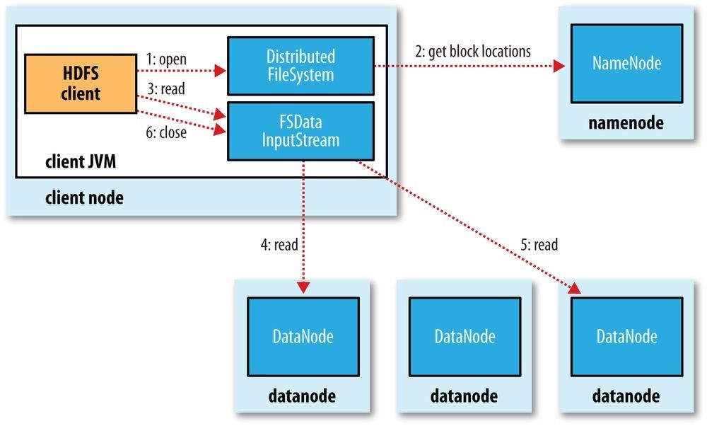
Figure 3-2. A client reading data from HDFS
The client opens the file it wishes to read by calling open() on the FileSystem object, which for HDFS is an instance of DistributedFileSystem (step 1 in Figure 3-2). DistributedFileSystem calls the namenode, using remote procedure calls (RPCs), to determine the locations of the first few blocks in the file (step 2). For each block, the namenode returns the addresses of the datanodes that have a copy of that block.
Furthermore, the datanodes are sorted according to their proximity to the client (according to the topology of the cluster’s network; see Network Topology and Hadoop). If the client is itself a datanode (in the case of a MapReduce task, for instance), the client will read from the local datanode if that datanode hosts a copy of the block (see also Figure 2-2 and Short-circuit local reads).
The DistributedFileSystem returns an FSDataInputStream (an input stream that supports file seeks) to the client for it to read data from. FSDataInputStream in turn wraps a DFSInputStream, which manages the datanode and namenode I/O.
The client then calls read() on the stream (step 3). DFSInputStream, which has stored the datanode addresses for the first few blocks in the file, then connects to the first (closest) datanode for the first block in the file. Data is streamed from the datanode back to the client, which calls read() repeatedly on the stream (step 4). When the end of the block is reached, DFSInputStream will close the connection to the datanode, then find the best datanode for the next block (step 5). This happens transparently to the client, which from its point of view is just reading a continuous stream.
Blocks are read in order, with the DFSInputStream opening new connections to datanodes as the client reads through the stream. It will also call the namenode to retrieve the datanode locations for the next batch of blocks as needed. When the client has finished reading, it calls close() on the FSDataInputStream (step 6).
During reading, if the DFSInputStream encounters an error while communicating with a datanode, it will try the next closest one for that block. It will also remember datanodes that have failed so that it doesn’t needlessly retry them for later blocks. The
DFSInputStream also verifies checksums for the data transferred to it from the datanode. If a corrupted block is found, the DFSInputStream attempts to read a replica of the block from another datanode; it also reports the corrupted block to the namenode.
One important aspect of this design is that the client contacts datanodes directly to retrieve data and is guided by the namenode to the best datanode for each block. This design allows HDFS to scale to a large number of concurrent clients because the data traffic is spread across all the datanodes in the cluster. Meanwhile, the namenode merely has to service block location requests (which it stores in memory, making them very efficient) and does not, for example, serve data, which would quickly become a bottleneck as the number of clients grew.
NETWORK TOPOLOGY AND HADOOP
What does it mean for two nodes in a local network to be “close” to each other? In the context of high-volume data processing, the limiting factor is the rate at which we can transfer data between nodes — bandwidth is a scarce commodity. The idea is to use the bandwidth between two nodes as a measure of distance.
Rather than measuring bandwidth between nodes, which can be difficult to do in practice (it requires a quiet cluster, and the number of pairs of nodes in a cluster grows as the square of the number of nodes), Hadoop takes a simple approach in which the network is represented as a tree and the distance between two nodes is the sum of their distances to their closest common ancestor. Levels in the tree are not predefined, but it is common to have levels that correspond to the data center, the rack, and the node that a process is running on. The idea is that the bandwidth available for each of the following scenarios becomes progressively less:
Processes on the same node
Different nodes on the same rack
Nodes on different racks in the same data center
Nodes in different data centers[32]
For example, imagine a node n1 on rack r1 in data center d1. This can be represented as /d1/r1/n1. Using this notation, here are the distances for the four scenarios:
distance(/d1/r1/n1, /d1/r1/n1) = 0 (processes on the same node) distance(/d1/r1/n1, /d1/r1/n2) = 2 (different nodes on the same rack)
distance(/d1/r1/n1, /d1/r2/n3) = 4 (nodes on different racks in the same data center) distance(/d1/r1/n1, /d2/r3/n4) = 6 (nodes in different data centers)
This is illustrated schematically in Figure 3-3. (Mathematically inclined readers will notice that this is an example of a distance metric.)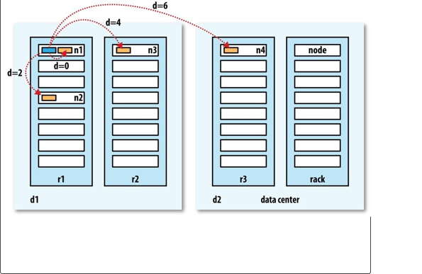
Anatomy of a File Write
Next we’ll look at how files are written to HDFS. Although quite detailed, it is instructive to understand the data flow because it clarifies HDFS’s coherency model.
We’re going to consider the case of creating a new file, writing data to it, then closing the file. This is illustrated in Figure 3-4.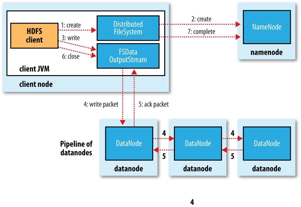
Figure 3-4. A client writing data to HDFS
The client creates the file by calling create() on DistributedFileSystem (step 1 in Figure 3-4). DistributedFileSystem makes an RPC call to the namenode to create a new file in the filesystem’s namespace, with no blocks associated with it (step 2). The namenode performs various checks to make sure the file doesn’t already exist and that the client has the right permissions to create the file. If these checks pass, the namenode makes a record of the new file; otherwise, file creation fails and the client is thrown an
IOException. The DistributedFileSystem returns an FSDataOutputStream for the client
to start writing data to. Just as in the read case, FSDataOutputStream wraps a DFSOutputStream, which handles communication with the datanodes and namenode.
As the client writes data (step 3), the DFSOutputStream splits it into packets, which it writes to an internal queue called the data queue. The data queue is consumed by the DataStreamer, which is responsible for asking the namenode to allocate new blocks by picking a list of suitable datanodes to store the replicas. The list of datanodes forms a pipeline, and here we’ll assume the replication level is three, so there are three nodes in the pipeline. The DataStreamer streams the packets to the first datanode in the pipeline, which stores each packet and forwards it to the second datanode in the pipeline. Similarly, the second datanode stores the packet and forwards it to the third (and last) datanode in the pipeline (step 4).
The DFSOutputStream also maintains an internal queue of packets that are waiting to be acknowledged by datanodes, called the ack queue. A packet is removed from the ack queue only when it has been acknowledged by all the datanodes in the pipeline (step 5).
If any datanode fails while data is being written to it, then the following actions are taken, which are transparent to the client writing the data. First, the pipeline is closed, and any packets in the ack queue are added to the front of the data queue so that datanodes that are downstream from the failed node will not miss any packets. The current block on the good datanodes is given a new identity, which is communicated to the namenode, so that the partial block on the failed datanode will be deleted if the failed datanode recovers later on. The failed datanode is removed from the pipeline, and a new pipeline is constructed from the two good datanodes. The remainder of the block’s data is written to the good datanodes in the pipeline. The namenode notices that the block is under-replicated, and it arranges for a further replica to be created on another node. Subsequent blocks are then treated as normal.
It’s possible, but unlikely, for multiple datanodes to fail while a block is being written. As long as dfs.namenode.replication.min replicas (which defaults to 1) are written, the write will succeed, and the block will be asynchronously replicated across the cluster until its target replication factor is reached (dfs.replication, which defaults to 3).
When the client has finished writing data, it calls close() on the stream (step 6). This action flushes all the remaining packets to the datanode pipeline and waits for
acknowledgments before contacting the namenode to signal that the file is complete (step
7). The namenode already knows which blocks the file is made up of (because
DataStreamer asks for block allocations), so it only has to wait for blocks to be minimally replicated before returning successfully.
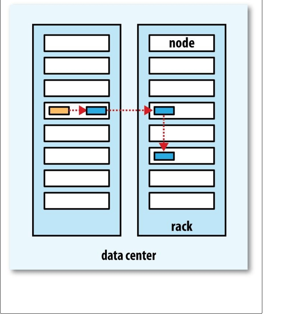
Coherency Model
A coherency model for a filesystem describes the data visibility of reads and writes for a file. HDFS trades off some POSIX requirements for performance, so some operations may behave differently than you expect them to.
After creating a file, it is visible in the filesystem namespace, as expected:
Path p = new Path(“p”); fs.create(p); assertThat(fs.exists(p), is(true));
However, any content written to the file is not guaranteed to be visible, even if the stream is flushed. So, the file appears to have a length of zero:
Path p = new Path(“p”);
OutputStream out = fs.create(p); out.write(“content”.getBytes(“UTF-8”)); out.flush(); assertThat(fs.getFileStatus(p).getLen(), is(0L));
Once more than a block’s worth of data has been written, the first block will be visible to new readers. This is true of subsequent blocks, too: it is always the current block being written that is not visible to other readers.
HDFS provides a way to force all buffers to be flushed to the datanodes via the hflush() method on FSDataOutputStream. After a successful return from hflush(), HDFS guarantees that the data written up to that point in the file has reached all the datanodes in the write pipeline and is visible to all new readers:
Path p = new Path(“p”);
FSDataOutputStream out = fs.create(p); out.write(“content”.getBytes(“UTF-8”)); out.hflush(); assertThat(fs.getFileStatus(p).getLen(), is(((long) “content”.length())));
Note that hflush() does not guarantee that the datanodes have written the data to disk, only that it’s in the datanodes’ memory (so in the event of a data center power outage, for example, data could be lost). For this stronger guarantee, use hsync() instead.33]
The behavior of hsync() is similar to that of the fsync() system call in POSIX that commits buffered data for a file descriptor. For example, using the standard Java API to write a local file, we are guaranteed to see the content after flushing the stream and synchronizing:
FileOutputStream out = new FileOutputStream(localFile); out.write(“content”.getBytes(“UTF-8”)); out.flush(); // flush to operating system out.getFD().sync(); // sync to disk assertThat(localFile.length(), is(((long) “content”.length()))); Closing a file in HDFS performs an implicit hflush(), too:
Path p = new Path(“p”);
OutputStream out = fs.create(p); out.write(“content”.getBytes(“UTF-8”)); out.close(); assertThat(fs.getFileStatus(p).getLen(), is(((long) “content”.length())));
Consequences for application design
This coherency model has implications for the way you design applications. With no calls to hflush() or hsync(), you should be prepared to lose up to a block of data in the event of client or system failure. For many applications, this is unacceptable, so you should call hflush() at suitable points, such as after writing a certain number of records or number of bytes. Though the hflush() operation is designed to not unduly tax HDFS, it does have some overhead (and hsync() has more), so there is a trade-off between data robustness and throughput. What constitutes an acceptable trade-off is application dependent, and suitable values can be selected after measuring your application’s performance with different hflush() (or hsync()) frequencies.
Parallel Copying with distcp
The HDFS access patterns that we have seen so far focus on single-threaded access. It’s possible to act on a collection of files — by specifying file globs, for example — but for efficient parallel processing of these files, you would have to write a program yourself. Hadoop comes with a useful program called distcp for copying data to and from Hadoop filesystems in parallel.
One use for distcp is as an efficient replacement for hadoop fs -cp. For example, you can copy one file to another with:34]
% hadoop distcp file1 file2 You can also copy directories:
% hadoop distcp dir1 dir2
If dir2 does not exist, it will be created, and the contents of the dir1 directory will be copied there. You can specify multiple source paths, and all will be copied to the destination.
If dir2 already exists, then dir1 will be copied under it, creating the directory structure dir2/dir1. If this isn’t what you want, you can supply the -overwrite option to keep the same directory structure and force files to be overwritten. You can also update only the files that have changed using the -update option. This is best shown with an example. If we changed a file in the dir1 subtree, we could synchronize the change with dir2 by running:
% hadoop distcp -update dir1 dir2
distcp is implemented as a MapReduce job where the work of copying is done by the maps that run in parallel across the cluster. There are no reducers. Each file is copied by a single map, and distcp tries to give each map approximately the same amount of data by bucketing files into roughly equal allocations. By default, up to 20 maps are used, but this can be changed by specifying the -m argument to distcp.
A very common use case for distcp is for transferring data between two HDFS clusters. For example, the following creates a backup of the first cluster’s /foo directory on the second:
% hadoop distcp -update -delete -p hdfs://namenode1/foo hdfs://namenode2/foo
The -delete flag causes distcp to delete any files or directories from the destination that are not present in the source, and -p means that file status attributes like permissions, block size, and replication are preserved. You can run distcp with no arguments to see precise usage instructions.
If the two clusters are running incompatible versions of HDFS, then you can use the webhdfs protocol to distcp between them:
% hadoop distcp webhdfs://namenode1:50070/foo webhdfs://namenode2:50070/foo
Another variant is to use an HttpFs proxy as the distcp source or destination (again using the webhdfs protocol), which has the advantage of being able to set firewall and bandwidth controls (see HTTP).
Keeping an HDFS Cluster Balanced
When copying data into HDFS, it’s important to consider cluster balance. HDFS works best when the file blocks are evenly spread across the cluster, so you want to ensure that distcp doesn’t disrupt this. For example, if you specified -m 1, a single map would do the copy, which — apart from being slow and not using the cluster resources efficiently — would mean that the first replica of each block would reside on the node running the map (until the disk filled up). The second and third replicas would be spread across the cluster, but this one node would be unbalanced. By having more maps than nodes in the cluster, this problem is avoided. For this reason, it’s best to start by running distcp with the default of 20 maps per node.
However, it’s not always possible to prevent a cluster from becoming unbalanced. Perhaps you want to limit the number of maps so that some of the nodes can be used by other jobs. In this case, you can use the balancer tool (see Balancer) to subsequently even out the block distribution across the cluster.
[25] The architecture of HDFS is described in Robert Chansler et al.’s, “The Hadoop Distributed File System,” which appeared in The Architecture of Open Source Applications: Elegance, Evolution, and a Few Fearless Hacks by Amy Brown and Greg Wilson (eds.).
[26] See Konstantin V. Shvachko and Arun C. Murthy, “Scaling Hadoop to 4000 nodes at Yahoo!”, September 30, 2008.
[27] See Chapter 10 for a typical machine specification.
[28] For an exposition of the scalability limits of HDFS, see Konstantin V. Shvachko, “HDFS Scalability: The Limits to Growth”, April 2010.
[29] In Hadoop 1, the name for this property was fs.default.name. Hadoop 2 introduced many new property names, and deprecated the old ones (see Which Properties Can I Set?). This book uses the new property names.
[30] In Hadoop 2 and later, there is a new filesystem interface called FileContext with better handling of multiple filesystems (so a single FileContext can resolve multiple filesystem schemes, for example) and a cleaner, more consistent interface. FileSystem is still more widely used, however.
[31] The text is from The Quangle Wangle’s Hat by Edward Lear.
[32] At the time of this writing, Hadoop is not suited for running across data centers.
[33] In Hadoop 1.x, hflush() was called sync(), and hsync() did not exist.
[34] Even for a single file copy, the distcp variant is preferred for large files since hadoop fs -cp copies the file via the client running the command.
Chapter 4. YARN
Apache YARN (Yet Another Resource Negotiator) is Hadoop’s cluster resource management system. YARN was introduced in Hadoop 2 to improve the MapReduce implementation, but it is general enough to support other distributed computing paradigms as well.
YARN provides APIs for requesting and working with cluster resources, but these APIs are not typically used directly by user code. Instead, users write to higher-level APIs provided by distributed computing frameworks, which themselves are built on YARN and hide the resource management details from the user. The situation is illustrated in Figure 4-1, which shows some distributed computing frameworks (MapReduce, Spark, and so on) running as YARN applications on the cluster compute layer (YARN) and the cluster storage layer (HDFS and HBase).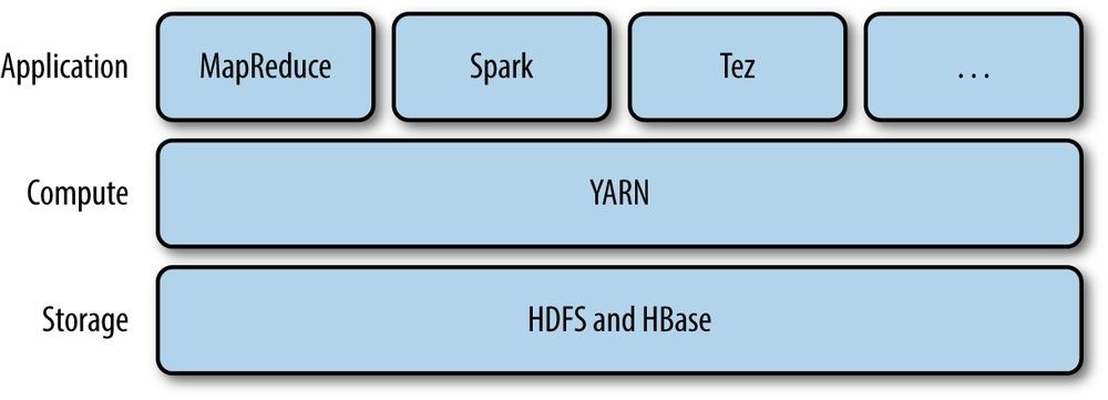
Figure 4-1. YARN applications
There is also a layer of applications that build on the frameworks shown in Figure 4-1. Pig, Hive, and Crunch are all examples of processing frameworks that run on MapReduce, Spark, or Tez (or on all three), and don’t interact with YARN directly.
This chapter walks through the features in YARN and provides a basis for understanding later chapters in Part IV that cover Hadoop’s distributed processing frameworks.
Anatomy of a YARN Application Run
YARN provides its core services via two types of long-running daemon: a resource manager (one per cluster) to manage the use of resources across the cluster, and node managers running on all the nodes in the cluster to launch and monitor containers. A container executes an application-specific process with a constrained set of resources (memory, CPU, and so on). Depending on how YARN is configured (see YARN), a container may be a Unix process or a Linux cgroup. Figure 4-2 illustrates how YARN runs an application.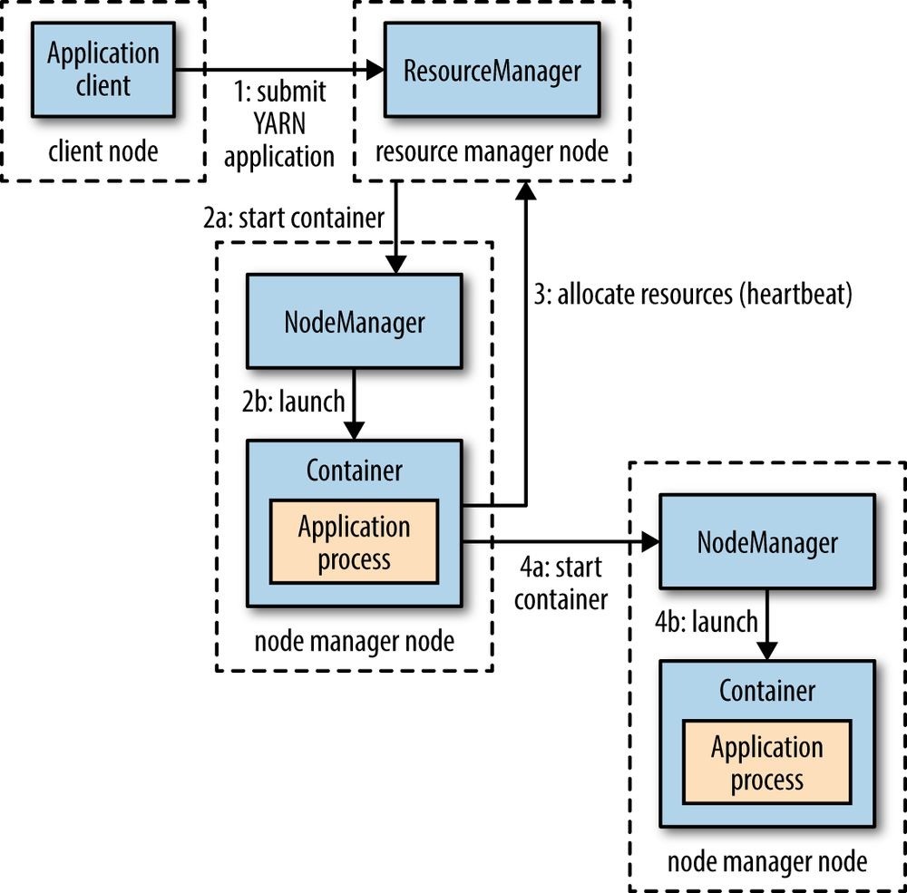
Figure 4-2. How YARN runs an application
To run an application on YARN, a client contacts the resource manager and asks it to run an application master process (step 1 in Figure 4-2). The resource manager then finds a node manager that can launch the application master in a container (steps 2a and 2b).35] Precisely what the application master does once it is running depends on the application. It could simply run a computation in the container it is running in and return the result to the client. Or it could request more containers from the resource managers (step 3), and use them to run a distributed computation (steps 4a and 4b). The latter is what the MapReduce YARN application does, which we’ll look at in more detail in Anatomy of a MapReduce Job Run.
Notice from Figure 4-2 that YARN itself does not provide any way for the parts of the application (client, master, process) to communicate with one another. Most nontrivial YARN applications use some form of remote communication (such as Hadoop’s RPC layer) to pass status updates and results back to the client, but these are specific to the application.
Resource Requests
YARN has a flexible model for making resource requests. A request for a set of containers can express the amount of computer resources required for each container (memory and CPU), as well as locality constraints for the containers in that request.
Locality is critical in ensuring that distributed data processing algorithms use the cluster bandwidth efficiently,36] so YARN allows an application to specify locality constraints for the containers it is requesting. Locality constraints can be used to request a container on a specific node or rack, or anywhere on the cluster (off-rack).
Sometimes the locality constraint cannot be met, in which case either no allocation is made or, optionally, the constraint can be loosened. For example, if a specific node was requested but it is not possible to start a container on it (because other containers are running on it), then YARN will try to start a container on a node in the same rack, or, if that’s not possible, on any node in the cluster.
In the common case of launching a container to process an HDFS block (to run a map task in MapReduce, say), the application will request a container on one of the nodes hosting the block’s three replicas, or on a node in one of the racks hosting the replicas, or, failing that, on any node in the cluster.
A YARN application can make resource requests at any time while it is running. For example, an application can make all of its requests up front, or it can take a more dynamic approach whereby it requests more resources dynamically to meet the changing needs of the application.
Spark takes the first approach, starting a fixed number of executors on the cluster (see
Spark on YARN). MapReduce, on the other hand, has two phases: the map task containers are requested up front, but the reduce task containers are not started until later. Also, if any tasks fail, additional containers will be requested so the failed tasks can be rerun.
Application Lifespan
The lifespan of a YARN application can vary dramatically: from a short-lived application of a few seconds to a long-running application that runs for days or even months. Rather than look at how long the application runs for, it’s useful to categorize applications in terms of how they map to the jobs that users run. The simplest case is one application per user job, which is the approach that MapReduce takes.
The second model is to run one application per workflow or user session of (possibly unrelated) jobs. This approach can be more efficient than the first, since containers can be reused between jobs, and there is also the potential to cache intermediate data between jobs. Spark is an example that uses this model.
The third model is a long-running application that is shared by different users. Such an application often acts in some kind of coordination role. For example, Apache Slider has a long-running application master for launching other applications on the cluster. This approach is also used by Impala (see SQL-on-Hadoop Alternatives) to provide a proxy application that the Impala daemons communicate with to request cluster resources. The “always on” application master means that users have very low-latency responses to their queries since the overhead of starting a new application master is avoided.37]
Building YARN Applications
Writing a YARN application from scratch is fairly involved, but in many cases is not necessary, as it is often possible to use an existing application that fits the bill. For example, if you are interested in running a directed acyclic graph (DAG) of jobs, then Spark or Tez is appropriate; or for stream processing, Spark, Samza, or Storm works.38]
There are a couple of projects that simplify the process of building a YARN application. Apache Slider, mentioned earlier, makes it possible to run existing distributed applications on YARN. Users can run their own instances of an application (such as HBase) on a cluster, independently of other users, which means that different users can run different versions of the same application. Slider provides controls to change the number of nodes an application is running on, and to suspend then resume a running application.
Apache Twill is similar to Slider, but in addition provides a simple programming model for developing distributed applications on YARN. Twill allows you to define cluster processes as an extension of a Java Runnable, then runs them in YARN containers on the cluster. Twill also provides support for, among other things, real-time logging (log events from runnables are streamed back to the client) and command messages (sent from the client to runnables).
In cases where none of these options are sufficient — such as an application that has complex scheduling requirements — then the distributed shell application that is a part of the YARN project itself serves as an example of how to write a YARN application. It demonstrates how to use YARN’s client APIs to handle communication between the client or application master and the YARN daemons.
YARN Compared to MapReduce 1
The distributed implementation of MapReduce in the original version of Hadoop (version 1 and earlier) is sometimes referred to as “MapReduce 1” to distinguish it from MapReduce 2, the implementation that uses YARN (in Hadoop 2 and later).
NOTE
It’s important to realize that the old and new MapReduce APIs are not the same thing as the MapReduce 1 and
MapReduce 2 implementations. The APIs are user-facing client-side features and determine how you write
MapReduce programs (see Appendix D), whereas the implementations are just different ways of running MapReduce programs. All four combinations are supported: both the old and new MapReduce APIs run on both MapReduce 1 and 2.
In MapReduce 1, there are two types of daemon that control the job execution process: a jobtracker and one or more tasktrackers. The jobtracker coordinates all the jobs run on the system by scheduling tasks to run on tasktrackers. Tasktrackers run tasks and send progress reports to the jobtracker, which keeps a record of the overall progress of each job. If a task fails, the jobtracker can reschedule it on a different tasktracker.
In MapReduce 1, the jobtracker takes care of both job scheduling (matching tasks with tasktrackers) and task progress monitoring (keeping track of tasks, restarting failed or slow tasks, and doing task bookkeeping, such as maintaining counter totals). By contrast, in YARN these responsibilities are handled by separate entities: the resource manager and an application master (one for each MapReduce job). The jobtracker is also responsible for storing job history for completed jobs, although it is possible to run a job history server as a separate daemon to take the load off the jobtracker. In YARN, the equivalent role is the timeline server, which stores application history.39]
The YARN equivalent of a tasktracker is a node manager. The mapping is summarized in Table 4-1.
Table 4-1. A comparison of MapReduce 1 and YARN components
MapReduce 1 YARN
| Jobtracker | Resource manager, application master, timeline server |
|---|---|
| Tasktracker | Node manager |
| Slot | Container |
YARN was designed to address many of the limitations in MapReduce 1. The benefits to using YARN include the following:
Scalability
YARN can run on larger clusters than MapReduce 1. MapReduce 1 hits scalability bottlenecks in the region of 4,000 nodes and 40,000 tasks,40] stemming from the fact that the jobtracker has to manage both jobs and tasks. YARN overcomes these limitations by virtue of its split resource manager/application master architecture: it is designed to scale up to 10,000 nodes and 100,000 tasks.
In contrast to the jobtracker, each instance of an application — here, a MapReduce job — has a dedicated application master, which runs for the duration of the application. This model is actually closer to the original Google MapReduce paper, which describes how a master process is started to coordinate map and reduce tasks running on a set of workers.
Availability
High availability (HA) is usually achieved by replicating the state needed for another daemon to take over the work needed to provide the service, in the event of the service daemon failing. However, the large amount of rapidly changing complex state in the jobtracker’s memory (each task status is updated every few seconds, for example) makes it very difficult to retrofit HA into the jobtracker service.
With the jobtracker’s responsibilities split between the resource manager and application master in YARN, making the service highly available became a divide-andconquer problem: provide HA for the resource manager, then for YARN applications (on a per-application basis). And indeed, Hadoop 2 supports HA both for the resource manager and for the application master for MapReduce jobs. Failure recovery in YARN is discussed in more detail in Failures.
Utilization
In MapReduce 1, each tasktracker is configured with a static allocation of fixed-size “slots,” which are divided into map slots and reduce slots at configuration time. A map slot can only be used to run a map task, and a reduce slot can only be used for a reduce task.
In YARN, a node manager manages a pool of resources, rather than a fixed number of designated slots. MapReduce running on YARN will not hit the situation where a reduce task has to wait because only map slots are available on the cluster, which can happen in MapReduce 1. If the resources to run the task are available, then the application will be eligible for them.
Furthermore, resources in YARN are fine grained, so an application can make a request for what it needs, rather than for an indivisible slot, which may be too big (which is wasteful of resources) or too small (which may cause a failure) for the particular task.
Multitenancy
In some ways, the biggest benefit of YARN is that it opens up Hadoop to other types of distributed application beyond MapReduce. MapReduce is just one YARN application among many.
It is even possible for users to run different versions of MapReduce on the same YARN cluster, which makes the process of upgrading MapReduce more manageable. (Note, however, that some parts of MapReduce, such as the job history server and the shuffle handler, as well as YARN itself, still need to be upgraded across the cluster.)
Since Hadoop 2 is widely used and is the latest stable version, in the rest of this book the term “MapReduce” refers to MapReduce 2 unless otherwise stated. Chapter 7 looks in detail at how MapReduce running on YARN works.
Scheduling in YARN
In an ideal world, the requests that a YARN application makes would be granted immediately. In the real world, however, resources are limited, and on a busy cluster, an application will often need to wait to have some of its requests fulfilled. It is the job of the YARN scheduler to allocate resources to applications according to some defined policy. Scheduling in general is a difficult problem and there is no one “best” policy, which is why YARN provides a choice of schedulers and configurable policies. We look at these next.
Scheduler Options
Three schedulers are available in YARN: the FIFO, Capacity, and Fair Schedulers. The
FIFO Scheduler places applications in a queue and runs them in the order of submission (first in, first out). Requests for the first application in the queue are allocated first; once its requests have been satisfied, the next application in the queue is served, and so on.
The FIFO Scheduler has the merit of being simple to understand and not needing any configuration, but it’s not suitable for shared clusters. Large applications will use all the resources in a cluster, so each application has to wait its turn. On a shared cluster it is better to use the Capacity Scheduler or the Fair Scheduler. Both of these allow longrunning jobs to complete in a timely manner, while still allowing users who are running concurrent smaller ad hoc queries to get results back in a reasonable time.
The difference between schedulers is illustrated in Figure 4-3, which shows that under the FIFO Scheduler (i) the small job is blocked until the large job completes.
With the Capacity Scheduler (ii in Figure 4-3), a separate dedicated queue allows the small job to start as soon as it is submitted, although this is at the cost of overall cluster utilization since the queue capacity is reserved for jobs in that queue. This means that the large job finishes later than when using the FIFO Scheduler.
With the Fair Scheduler (iii in Figure 4-3), there is no need to reserve a set amount of capacity, since it will dynamically balance resources between all running jobs. Just after the first (large) job starts, it is the only job running, so it gets all the resources in the cluster. When the second (small) job starts, it is allocated half of the cluster resources so that each job is using its fair share of resources.
Note that there is a lag between the time the second job starts and when it receives its fair share, since it has to wait for resources to free up as containers used by the first job complete. After the small job completes and no longer requires resources, the large job goes back to using the full cluster capacity again. The overall effect is both high cluster utilization and timely small job completion.
Figure 4-3 contrasts the basic operation of the three schedulers. In the next two sections, we examine some of the more advanced configuration options for the Capacity and Fair Schedulers.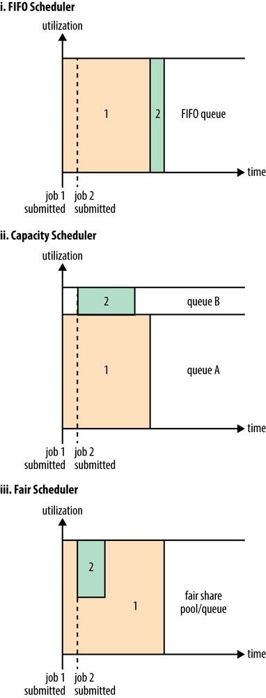
Figure 4-3. Cluster utilization over time when running a large job and a small job under the FIFO Scheduler (i),
Capacity Scheduler (ii), and Fair Scheduler (iii)
Capacity Scheduler Configuration
The Capacity Scheduler allows sharing of a Hadoop cluster along organizational lines, whereby each organization is allocated a certain capacity of the overall cluster. Each organization is set up with a dedicated queue that is configured to use a given fraction of the cluster capacity. Queues may be further divided in hierarchical fashion, allowing each organization to share its cluster allowance between different groups of users within the organization. Within a queue, applications are scheduled using FIFO scheduling.
As we saw in Figure 4-3, a single job does not use more resources than its queue’s capacity. However, if there is more than one job in the queue and there are idle resources available, then the Capacity Scheduler may allocate the spare resources to jobs in the queue, even if that causes the queue’s capacity to be exceeded.41] This behavior is known as queue elasticity.
In normal operation, the Capacity Scheduler does not preempt containers by forcibly killing them,42] so if a queue is under capacity due to lack of demand, and then demand increases, the queue will only return to capacity as resources are released from other queues as containers complete. It is possible to mitigate this by configuring queues with a maximum capacity so that they don’t eat into other queues’ capacities too much. This is at the cost of queue elasticity, of course, so a reasonable trade-off should be found by trial and error.
Imagine a queue hierarchy that looks like this:
root ├── prod
└── dev
├── eng
└── science
The listing in Example 4-1 shows a sample Capacity Scheduler configuration file, called capacity-scheduler.xml, for this hierarchy. It defines two queues under the root queue, prod and dev, which have 40% and 60% of the capacity, respectively. Notice that a particular queue is configured by setting configuration properties of the form
yarn.scheduler.capacity.
Example 4-1. A basic configuration file for the Capacity Scheduler
<?xml version=”1.0”?>
As you can see, the dev queue is further divided into eng and science queues of equal capacity. So that the dev queue does not use up all the cluster resources when the prod queue is idle, it has its maximum capacity set to 75%. In other words, the prod queue always has 25% of the cluster available for immediate use. Since no maximum capacities have been set for other queues, it’s possible for jobs in the eng or science queues to use all of the dev queue’s capacity (up to 75% of the cluster), or indeed for the prod queue to use the entire cluster.
Beyond configuring queue hierarchies and capacities, there are settings to control the maximum number of resources a single user or application can be allocated, how many applications can be running at any one time, and ACLs on queues. See the reference page for details.
Queue placement
The way that you specify which queue an application is placed in is specific to the application. For example, in MapReduce, you set the property mapreduce.job.queuename to the name of the queue you want to use. If the queue does not exist, then you’ll get an error at submission time. If no queue is specified, applications will be placed in a queue called default.
WARNING
For the Capacity Scheduler, the queue name should be the last part of the hierarchical name since the full hierarchical name is not recognized. So, for the preceding example configuration, prod and eng are OK, but root.dev.eng and dev.eng do not work.
Fair Scheduler Configuration
The Fair Scheduler attempts to allocate resources so that all running applications get the same share of resources. Figure 4-3 showed how fair sharing works for applications in the same queue; however, fair sharing actually works between queues, too, as we’ll see next.
To understand how resources are shared between queues, imagine two users A and B, each with their own queue (Figure 4-4). A starts a job, and it is allocated all the resources available since there is no demand from B. Then B starts a job while A’s job is still running, and after a while each job is using half of the resources, in the way we saw earlier. Now if B starts a second job while the other jobs are still running, it will share its resources with B’s other job, so each of B’s jobs will have one-fourth of the resources, while A’s will continue to have half. The result is that resources are shared fairly between users.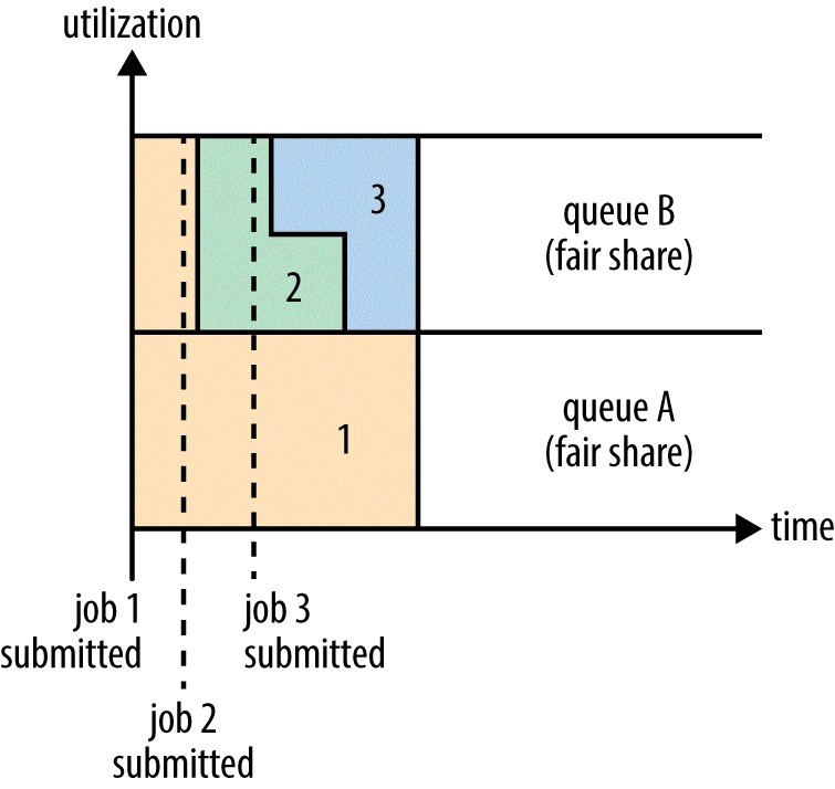
Figure 4-4. Fair sharing between user queues
Enabling the Fair Scheduler
The scheduler in use is determined by the setting of yarn.resourcemanager.scheduler.class. The Capacity Scheduler is used by default (although the Fair Scheduler is the default in some Hadoop distributions, such as CDH), but this can be changed by setting yarn.resourcemanager.scheduler.class in yarnsite.xml to the fully qualified classname of the scheduler, org.apache.hadoop.yarn.server.resourcemanager.scheduler.fair.FairScheduler.
Queue configuration
The Fair Scheduler is configured using an allocation file named fair-scheduler.xml that is loaded from the classpath. (The name can be changed by setting the property yarn.scheduler.fair.allocation.file.) In the absence of an allocation file, the Fair Scheduler operates as described earlier: each application is placed in a queue named after the user and queues are created dynamically when users submit their first applications.
Per-queue configuration is specified in the allocation file. This allows configuration of hierarchical queues like those supported by the Capacity Scheduler. For example, we can define prod and dev queues like we did for the Capacity Scheduler using the allocation file in Example 4-2.
Example 4-2. An allocation file for the Fair Scheduler
<?xml version=”1.0”?>
<queue name=”prod”>
<queue name=”dev”>
<queue name=”eng” />
<queue name=”science” />
<rule name=”specified” create=”false” />
<rule name=”primaryGroup” create=”false” />
<rule name=”default” queue=”dev.eng” />
The queue hierarchy is defined using nested queue elements. All queues are children of the root queue, even if not actually nested in a root queue element. Here we subdivide the dev queue into a queue called eng and another called science.
Queues can have weights, which are used in the fair share calculation. In this example, the cluster allocation is considered fair when it is divided into a 40:60 proportion between prod and dev. The eng and science queues do not have weights specified, so they are divided evenly. Weights are not quite the same as percentages, even though the example uses numbers that add up to 100 for the sake of simplicity. We could have specified weights of 2 and 3 for the prod and dev queues to achieve the same queue weighting.
NOTE
When setting weights, remember to consider the default queue and dynamically created queues (such as queues named after users). These are not specified in the allocation file, but still have weight 1.
Queues can have different scheduling policies. The default policy for queues can be set in the top-level defaultQueueSchedulingPolicy element; if it is omitted, fair scheduling is used. Despite its name, the Fair Scheduler also supports a FIFO (fifo) policy on queues, as well as Dominant Resource Fairness (drf), described later in the chapter.
The policy for a particular queue can be overridden using the schedulingPolicy element for that queue. In this case, the prod queue uses FIFO scheduling since we want each production job to run serially and complete in the shortest possible amount of time. Note that fair sharing is still used to divide resources between the prod and dev queues, as well as between (and within) the eng and science queues.
Although not shown in this allocation file, queues can be configured with minimum and maximum resources, and a maximum number of running applications. (See the reference page for details.) The minimum resources setting is not a hard limit, but rather is used by the scheduler to prioritize resource allocations. If two queues are below their fair share, then the one that is furthest below its minimum is allocated resources first. The minimum resource setting is also used for preemption, discussed momentarily.
Queue placement
The Fair Scheduler uses a rules-based system to determine which queue an application is placed in. In Example 4-2, the queuePlacementPolicy element contains a list of rules, each of which is tried in turn until a match occurs. The first rule, specified, places an application in the queue it specified; if none is specified, or if the specified queue doesn’t exist, then the rule doesn’t match and the next rule is tried. The primaryGroup rule tries to place an application in a queue with the name of the user’s primary Unix group; if there is no such queue, rather than creating it, the next rule is tried. The default rule is a catch-all and always places the application in the dev.eng queue.
The queuePlacementPolicy can be omitted entirely, in which case the default behavior is as if it had been specified with the following:
<rule name=”specified” />
<rule name=”user” />
In other words, unless the queue is explicitly specified, the user’s name is used for the queue, creating it if necessary.
Another simple queue placement policy is one where all applications are placed in the same (default) queue. This allows resources to be shared fairly between applications, rather than users. The definition is equivalent to this:
<rule name=”default” />
It’s also possible to set this policy without using an allocation file, by setting yarn.scheduler.fair.user-as-default-queue to false so that applications will be placed in the default queue rather than a per-user queue. In addition, yarn.scheduler.fair.allow-undeclared-pools should be set to false so that users can’t create queues on the fly.
Preemption
When a job is submitted to an empty queue on a busy cluster, the job cannot start until resources free up from jobs that are already running on the cluster. To make the time taken for a job to start more predictable, the Fair Scheduler supports preemption.
Preemption allows the scheduler to kill containers for queues that are running with more than their fair share of resources so that the resources can be allocated to a queue that is under its fair share. Note that preemption reduces overall cluster efficiency, since the terminated containers need to be reexecuted.
Preemption is enabled globally by setting yarn.scheduler.fair.preemption to true. There are two relevant preemption timeout settings: one for minimum share and one for fair share, both specified in seconds. By default, the timeouts are not set, so you need to set at least one to allow containers to be preempted.
If a queue waits for as long as its minimum share preemption timeout without receiving its minimum guaranteed share, then the scheduler may preempt other containers. The default timeout is set for all queues via the defaultMinSharePreemptionTimeout top-level element in the allocation file, and on a per-queue basis by setting the minSharePreemptionTimeout element for a queue.
Likewise, if a queue remains below half of its fair share for as long as the fair share preemption timeout, then the scheduler may preempt other containers. The default timeout is set for all queues via the defaultFairSharePreemptionTimeout top-level element in the allocation file, and on a per-queue basis by setting fairSharePreemptionTimeout on a queue. The threshold may also be changed from its default of 0.5 by setting defaultFairSharePreemptionThreshold and fairSharePreemptionThreshold (perqueue).
Delay Scheduling
All the YARN schedulers try to honor locality requests. On a busy cluster, if an application requests a particular node, there is a good chance that other containers are running on it at the time of the request. The obvious course of action is to immediately loosen the locality requirement and allocate a container on the same rack. However, it has been observed in practice that waiting a short time (no more than a few seconds) can dramatically increase the chances of being allocated a container on the requested node, and therefore increase the efficiency of the cluster. This feature is called delay scheduling, and it is supported by both the Capacity Scheduler and the Fair Scheduler.
Every node manager in a YARN cluster periodically sends a heartbeat request to the resource manager — by default, one per second. Heartbeats carry information about the node manager’s running containers and the resources available for new containers, so each heartbeat is a potential scheduling opportunity for an application to run a container.
When using delay scheduling, the scheduler doesn’t simply use the first scheduling opportunity it receives, but waits for up to a given maximum number of scheduling opportunities to occur before loosening the locality constraint and taking the next scheduling opportunity.
For the Capacity Scheduler, delay scheduling is configured by setting yarn.scheduler.capacity.node-locality-delay to a positive integer representing the number of scheduling opportunities that it is prepared to miss before loosening the node constraint to match any node in the same rack.
The Fair Scheduler also uses the number of scheduling opportunities to determine the delay, although it is expressed as a proportion of the cluster size. For example, setting yarn.scheduler.fair.locality.threshold.node to 0.5 means that the scheduler should wait until half of the nodes in the cluster have presented scheduling opportunities before accepting another node in the same rack. There is a corresponding property, yarn.scheduler.fair.locality.threshold.rack, for setting the threshold before another rack is accepted instead of the one requested.
Dominant Resource Fairness
When there is only a single resource type being scheduled, such as memory, then the concept of capacity or fairness is easy to determine. If two users are running applications, you can measure the amount of memory that each is using to compare the two applications. However, when there are multiple resource types in play, things get more complicated. If one user’s application requires lots of CPU but little memory and the other’s requires little CPU and lots of memory, how are these two applications compared?
The way that the schedulers in YARN address this problem is to look at each user’s dominant resource and use it as a measure of the cluster usage. This approach is called
Dominant Resource Fairness, or DRF for short.43] The idea is best illustrated with a simple example.
Imagine a cluster with a total of 100 CPUs and 10 TB of memory. Application A requests containers of (2 CPUs, 300 GB), and application B requests containers of (6 CPUs, 100 GB). A’s request is (2%, 3%) of the cluster, so memory is dominant since its proportion (3%) is larger than CPU’s (2%). B’s request is (6%, 1%), so CPU is dominant. Since B’s container requests are twice as big in the dominant resource (6% versus 3%), it will be allocated half as many containers under fair sharing.
By default DRF is not used, so during resource calculations, only memory is considered and CPU is ignored. The Capacity Scheduler can be configured to use DRF by setting yarn.scheduler.capacity.resource-calculator to
org.apache.hadoop.yarn.util.resource.DominantResourceCalculator in capacityscheduler.xml.
For the Fair Scheduler, DRF can be enabled by setting the top-level element defaultQueueSchedulingPolicy in the allocation file to drf.
Further Reading
This chapter has given a short overview of YARN. For more detail, see Apache Hadoop YARN by Arun C. Murthy et al. (Addison-Wesley, 2014).
[35] It’s also possible for the client to start the application master, possibly outside the cluster, or in the same JVM as the client. This is called an unmanaged application master.
[36] For more on this topic see Scaling Out and Network Topology and Hadoop.
[37] The low-latency application master code lives in the Llama project.
[38] All of these projects are Apache Software Foundation projects.
[39] As of Hadoop 2.5.1, the YARN timeline server does not yet store MapReduce job history, so a MapReduce job history server daemon is still needed (see Cluster Setup and Installation).
[40] Arun C. Murthy, “The Next Generation of Apache Hadoop MapReduce,” February 14, 2011.
[41] If the property yarn.scheduler.capacity.
[42] However, the Capacity Scheduler can perform work-preserving preemption, where the resource manager asks applications to return containers to balance capacity.
[43] DRF was introduced in Ghodsi et al.’s “Dominant Resource Fairness: Fair Allocation of Multiple Resource Types,” March 2011.
Chapter 5. Hadoop I/O
Hadoop comes with a set of primitives for data I/O. Some of these are techniques that are more general than Hadoop, such as data integrity and compression, but deserve special consideration when dealing with multiterabyte datasets. Others are Hadoop tools or APIs that form the building blocks for developing distributed systems, such as serialization frameworks and on-disk data structures.
Data Integrity
Users of Hadoop rightly expect that no data will be lost or corrupted during storage or processing. However, because every I/O operation on the disk or network carries with it a small chance of introducing errors into the data that it is reading or writing, when the volumes of data flowing through the system are as large as the ones Hadoop is capable of handling, the chance of data corruption occurring is high.
The usual way of detecting corrupted data is by computing a checksum for the data when it first enters the system, and again whenever it is transmitted across a channel that is unreliable and hence capable of corrupting the data. The data is deemed to be corrupt if the newly generated checksum doesn’t exactly match the original. This technique doesn’t offer any way to fix the data — it is merely error detection. (And this is a reason for not using low-end hardware; in particular, be sure to use ECC memory.) Note that it is possible that it’s the checksum that is corrupt, not the data, but this is very unlikely, because the checksum is much smaller than the data.
A commonly used error-detecting code is CRC-32 (32-bit cyclic redundancy check), which computes a 32-bit integer checksum for input of any size. CRC-32 is used for checksumming in Hadoop’s ChecksumFileSystem, while HDFS uses a more efficient variant called CRC-32C.
Data Integrity in HDFS
HDFS transparently checksums all data written to it and by default verifies checksums when reading data. A separate checksum is created for every dfs.bytes-per-checksum bytes of data. The default is 512 bytes, and because a CRC-32C checksum is 4 bytes long, the storage overhead is less than 1%.
Datanodes are responsible for verifying the data they receive before storing the data and its checksum. This applies to data that they receive from clients and from other datanodes during replication. A client writing data sends it to a pipeline of datanodes (as explained in Chapter 3), and the last datanode in the pipeline verifies the checksum. If the datanode detects an error, the client receives a subclass of IOException, which it should handle in an application-specific manner (for example, by retrying the operation).
When clients read data from datanodes, they verify checksums as well, comparing them with the ones stored at the datanodes. Each datanode keeps a persistent log of checksum verifications, so it knows the last time each of its blocks was verified. When a client successfully verifies a block, it tells the datanode, which updates its log. Keeping statistics such as these is valuable in detecting bad disks.
In addition to block verification on client reads, each datanode runs a DataBlockScanner in a background thread that periodically verifies all the blocks stored on the datanode. This is to guard against corruption due to “bit rot” in the physical storage media. See Datanode block scanner for details on how to access the scanner reports.
Because HDFS stores replicas of blocks, it can “heal” corrupted blocks by copying one of the good replicas to produce a new, uncorrupt replica. The way this works is that if a client detects an error when reading a block, it reports the bad block and the datanode it was trying to read from to the namenode before throwing a ChecksumException. The namenode marks the block replica as corrupt so it doesn’t direct any more clients to it or try to copy this replica to another datanode. It then schedules a copy of the block to be replicated on another datanode, so its replication factor is back at the expected level. Once this has happened, the corrupt replica is deleted.
It is possible to disable verification of checksums by passing false to the
setVerifyChecksum() method on FileSystem before using the open() method to read a file. The same effect is possible from the shell by using the -ignoreCrc option with the get or the equivalent -copyToLocal command. This feature is useful if you have a corrupt file that you want to inspect so you can decide what to do with it. For example, you might want to see whether it can be salvaged before you delete it.
You can find a file’s checksum with hadoop fs -checksum. This is useful to check whether two files in HDFS have the same contents — something that distcp does, for example (see Parallel Copying with distcp).
LocalFileSystem
The Hadoop LocalFileSystem performs client-side checksumming. This means that when you write a file called filename, the filesystem client transparently creates a hidden file, .filename.crc, in the same directory containing the checksums for each chunk of the file.
The chunk size is controlled by the file.bytes-per-checksum property, which defaults to 512 bytes. The chunk size is stored as metadata in the .crc file, so the file can be read back correctly even if the setting for the chunk size has changed. Checksums are verified when the file is read, and if an error is detected, LocalFileSystem throws a ChecksumException.
Checksums are fairly cheap to compute (in Java, they are implemented in native code), typically adding a few percent overhead to the time to read or write a file. For most applications, this is an acceptable price to pay for data integrity. It is, however, possible to disable checksums, which is typically done when the underlying filesystem supports checksums natively. This is accomplished by using RawLocalFileSystem in place of LocalFileSystem. To do this globally in an application, it suffices to remap the implementation for file URIs by setting the property fs.file.impl to the value org.apache.hadoop.fs.RawLocalFileSystem. Alternatively, you can directly create a RawLocalFileSystem instance, which may be useful if you want to disable checksum verification for only some reads, for example:
Configuration conf = …
FileSystem fs = new RawLocalFileSystem(); fs.initialize(null, conf);
ChecksumFileSystem
LocalFileSystem uses ChecksumFileSystem to do its work, and this class makes it easy to add checksumming to other (nonchecksummed) filesystems, as ChecksumFileSystem is just a wrapper around FileSystem. The general idiom is as follows:
FileSystem rawFs = …
FileSystem checksummedFs = new ChecksumFileSystem(rawFs);
The underlying filesystem is called the raw filesystem, and may be retrieved using the getRawFileSystem() method on ChecksumFileSystem. ChecksumFileSystem has a few more useful methods for working with checksums, such as getChecksumFile() for getting the path of a checksum file for any file. Check the documentation for the others.
If an error is detected by ChecksumFileSystem when reading a file, it will call its reportChecksumFailure() method. The default implementation does nothing, but LocalFileSystem moves the offending file and its checksum to a side directory on the same device called bad_files. Administrators should periodically check for these bad files and take action on them.
Compression
File compression brings two major benefits: it reduces the space needed to store files, and it speeds up data transfer across the network or to or from disk. When dealing with large volumes of data, both of these savings can be significant, so it pays to carefully consider how to use compression in Hadoop.
There are many different compression formats, tools, and algorithms, each with different characteristics. Table 5-1 lists some of the more common ones that can be used with Hadoop.
Table 5-1. A summary of compression formats
| Compression format | Tool | Algorithm | Filename extension | Splittable? |
|---|---|---|---|---|
| DEFLATE[a] | N/A | DEFLATE | .deflate | No |
| gzip | gzip | DEFLATE | .gz | No |
| bzip2 | bzip2 | bzip2 | .bz2 | Yes |
| LZO | lzop | LZO | .lzo | No[b] |
| LZ4 | N/A | LZ4 | .lz4 | No |
| Snappy | N/A | Snappy | .snappy | No |
[a] DEFLATE is a compression algorithm whose standard implementation is zlib. There is no commonly available command-line tool for producing files in DEFLATE format, as gzip is normally used. (Note that the gzip file format is DEFLATE with extra headers and a footer.) The .deflate filename extension is a Hadoop convention.
[b] However, LZO files are splittable if they have been indexed in a preprocessing step. See Compression and Input Splits.
All compression algorithms exhibit a space/time trade-off: faster compression and decompression speeds usually come at the expense of smaller space savings. The tools listed in Table 5-1 typically give some control over this trade-off at compression time by offering nine different options: –1 means optimize for speed, and -9 means optimize for space. For example, the following command creates a compressed file file.gz using the fastest compression method:
% gzip -1 file
The different tools have very different compression characteristics. gzip is a generalpurpose compressor and sits in the middle of the space/time trade-off. bzip2 compresses more effectively than gzip, but is slower. bzip2’s decompression speed is faster than its compression speed, but it is still slower than the other formats. LZO, LZ4, and Snappy, on the other hand, all optimize for speed and are around an order of magnitude faster than gzip, but compress less effectively. Snappy and LZ4 are also significantly faster than LZO for decompression.44]
The “Splittable” column in Table 5-1 indicates whether the compression format supports splitting (that is, whether you can seek to any point in the stream and start reading from some point further on). Splittable compression formats are especially suitable for MapReduce; see Compression and Input Splits for further discussion.
Codecs
A codec is the implementation of a compression-decompression algorithm. In Hadoop, a codec is represented by an implementation of the CompressionCodec interface. So, for example, GzipCodec encapsulates the compression and decompression algorithm for gzip. Table 5-2 lists the codecs that are available for Hadoop.
Table 5-2. Hadoop compression codecs
Compression format Hadoop CompressionCodec
| DEFLATE | org.apache.hadoop.io.compress.DefaultCodec |
|---|---|
| gzip | org.apache.hadoop.io.compress.GzipCodec |
| bzip2 | org.apache.hadoop.io.compress.BZip2Codec |
| LZO | com.hadoop.compression.lzo.LzopCodec |
| LZ4 | org.apache.hadoop.io.compress.Lz4Codec |
| Snappy | org.apache.hadoop.io.compress.SnappyCodec |
The LZO libraries are GPL licensed and may not be included in Apache distributions, so for this reason the Hadoop codecs must be downloaded separately from Google (or
GitHub, which includes bug fixes and more tools). The LzopCodec, which is compatible with the lzop tool, is essentially the LZO format with extra headers, and is the one you normally want. There is also an LzoCodec for the pure LZO format, which uses the .lzo_deflate filename extension (by analogy with DEFLATE, which is gzip without the headers).
Compressing and decompressing streams with CompressionCodec
CompressionCodec has two methods that allow you to easily compress or decompress data. To compress data being written to an output stream, use the
createOutputStream(OutputStream out) method to create a CompressionOutputStream to which you write your uncompressed data to have it written in compressed form to the underlying stream. Conversely, to decompress data being read from an input stream, call createInputStream(InputStream in) to obtain a CompressionInputStream, which allows you to read uncompressed data from the underlying stream.
CompressionOutputStream and CompressionInputStream are similar to java.util.zip.DeflaterOutputStream and java.util.zip.DeflaterInputStream, except that both of the former provide the ability to reset their underlying compressor or decompressor. This is important for applications that compress sections of the data stream as separate blocks, such as in a SequenceFile, described in SequenceFile.
Example 5-1 illustrates how to use the API to compress data read from standard input and write it to standard output.
Example 5-1. A program to compress data read from standard input and write it to standard output
public class StreamCompressor {
public static void main(String[] args) throws Exception {
String codecClassname = args[0];
Class<?> codecClass = Class.forName(codecClassname); Configuration conf = new Configuration(); CompressionCodec codec = (CompressionCodec) ReflectionUtils.newInstance(codecClass, conf);
CompressionOutputStream out = codec.createOutputStream(System.out);
IOUtils.copyBytes(System.in, out, 4096, false); out.finish();
} }
The application expects the fully qualified name of the CompressionCodec implementation as the first command-line argument. We use ReflectionUtils to construct a new instance of the codec, then obtain a compression wrapper around System.out. Then we call the utility method copyBytes() on IOUtils to copy the input to the output, which is compressed by the CompressionOutputStream. Finally, we call finish() on CompressionOutputStream, which tells the compressor to finish writing to the compressed stream, but doesn’t close the stream. We can try it out with the following command line, which compresses the string “Text” using the StreamCompressor program with the GzipCodec, then decompresses it from standard input using gunzip:
% echo “Text” | hadoop StreamCompressor org.apache.hadoop.io.compress.GzipCodec \
| gunzip -
Text
Inferring CompressionCodecs using CompressionCodecFactory
If you are reading a compressed file, normally you can infer which codec to use by looking at its filename extension. A file ending in .gz can be read with GzipCodec, and so on. The extensions for each compression format are listed in Table 5-1.
CompressionCodecFactory provides a way of mapping a filename extension to a
CompressionCodec using its getCodec() method, which takes a Path object for the file in question. Example 5-2 shows an application that uses this feature to decompress files.
Example 5-2. A program to decompress a compressed file using a codec inferred from the file’s extension
public class FileDecompressor {
public static void main(String[] args) throws Exception {
String uri = args[0];
Configuration conf = new Configuration();
FileSystem fs = FileSystem.get(URI.create(uri), conf);
Path inputPath = new Path(uri);
CompressionCodecFactory factory = new CompressionCodecFactory(conf); CompressionCodec codec = factory.getCodec(inputPath); if (codec == null) {
System.err.println(“No codec found for “ + uri);
System.exit(1); }
String outputUri =
CompressionCodecFactory.removeSuffix(uri, codec.getDefaultExtension());
InputStream in = null; OutputStream out = null; try { in = codec.createInputStream(fs.open(inputPath)); out = fs.create(new Path(outputUri));
IOUtils.copyBytes(in, out, conf);
} finally {
IOUtils.closeStream(in);
IOUtils.closeStream(out);
}
} }
Once the codec has been found, it is used to strip off the file suffix to form the output filename (via the removeSuffix() static method of CompressionCodecFactory). In this way, a file named file.gz is decompressed to file by invoking the program as follows:
% hadoop FileDecompressor file.gz
CompressionCodecFactory loads all the codecs in Table 5-2, except LZO, as well as any listed in the io.compression.codecs configuration property (Table 5-3). By default, the property is empty; you would need to alter it only if you have a custom codec that you wish to register (such as the externally hosted LZO codecs). Each codec knows its default filename extension, thus permitting CompressionCodecFactory to search through the registered codecs to find a match for the given extension (if any).
Table 5-3. Compression codec properties
| Property name Type | Default value | Description |
|---|---|---|
| io.compression.codecs Comma-separated Class names | A list of additional CompressionCodec classes for compression/decompression |
Native libraries
For performance, it is preferable to use a native library for compression and decompression. For example, in one test, using the native gzip libraries reduced decompression times by up to 50% and compression times by around 10% (compared to the built-in Java implementation). Table 5-4 shows the availability of Java and native implementations for each compression format. All formats have native implementations, but not all have a Java implementation (LZO, for example).
Table 5-4. Compression library implementations
Compression format Java implementation? Native implementation?
| DEFLATE | Yes | Yes |
|---|---|---|
| gzip | Yes | Yes |
| bzip2 | Yes | Yes |
| LZO | No | Yes |
| LZ4 | No | Yes |
| Snappy | No | Yes |
The Apache Hadoop binary tarball comes with prebuilt native compression binaries for 64-bit Linux, called libhadoop.so. For other platforms, you will need to compile the libraries yourself, following the BUILDING.txt instructions at the top level of the source tree.
The native libraries are picked up using the Java system property java.library.path. The hadoop script in the etc/hadoop directory sets this property for you, but if you don’t use this script, you will need to set the property in your application.
By default, Hadoop looks for native libraries for the platform it is running on, and loads them automatically if they are found. This means you don’t have to change any configuration settings to use the native libraries. In some circumstances, however, you may wish to disable use of native libraries, such as when you are debugging a compression-related problem. You can do this by setting the property io.native.lib.available to false, which ensures that the built-in Java equivalents will be used (if they are available).
CodecPool
If you are using a native library and you are doing a lot of compression or decompression in your application, consider using CodecPool, which allows you to reuse compressors and decompressors, thereby amortizing the cost of creating these objects.
The code in Example 5-3 shows the API, although in this program, which creates only a single Compressor, there is really no need to use a pool.
Example 5-3. A program to compress data read from standard input and write it to standard output using a pooled compressor
public class PooledStreamCompressor {
public static void main(String[] args) throws Exception {
String codecClassname = args[0];
Class<?> codecClass = Class.forName(codecClassname);
Configuration conf = new Configuration();
CompressionCodec codec = (CompressionCodec)
ReflectionUtils.newInstance(codecClass, conf);
Compressor compressor = null; try {
compressor = CodecPool.getCompressor(codec); CompressionOutputStream out =
codec.createOutputStream(System.out, compressor);
IOUtils.copyBytes(System.in, out, 4096, false); out.finish();
} **finally {
CodecPool.returnCompressor(compressor); }**
} }
We retrieve a Compressor instance from the pool for a given CompressionCodec, which we use in the codec’s overloaded createOutputStream() method. By using a finally block, we ensure that the compressor is returned to the pool even if there is an IOException while copying the bytes between the streams.
Compression and Input Splits
When considering how to compress data that will be processed by MapReduce, it is important to understand whether the compression format supports splitting. Consider an uncompressed file stored in HDFS whose size is 1 GB. With an HDFS block size of 128 MB, the file will be stored as eight blocks, and a MapReduce job using this file as input will create eight input splits, each processed independently as input to a separate map task.
Imagine now that the file is a gzip-compressed file whose compressed size is 1 GB. As before, HDFS will store the file as eight blocks. However, creating a split for each block won’t work, because it is impossible to start reading at an arbitrary point in the gzip stream and therefore impossible for a map task to read its split independently of the others. The gzip format uses DEFLATE to store the compressed data, and DEFLATE stores data as a series of compressed blocks. The problem is that the start of each block is not distinguished in any way that would allow a reader positioned at an arbitrary point in the stream to advance to the beginning of the next block, thereby synchronizing itself with the stream. For this reason, gzip does not support splitting.
In this case, MapReduce will do the right thing and not try to split the gzipped file, since it knows that the input is gzip-compressed (by looking at the filename extension) and that gzip does not support splitting. This will work, but at the expense of locality: a single map will process the eight HDFS blocks, most of which will not be local to the map. Also, with fewer maps, the job is less granular and so may take longer to run.
If the file in our hypothetical example were an LZO file, we would have the same problem because the underlying compression format does not provide a way for a reader to synchronize itself with the stream. However, it is possible to preprocess LZO files using an indexer tool that comes with the Hadoop LZO libraries, which you can obtain from the Google and GitHub sites listed in Codecs. The tool builds an index of split points, effectively making them splittable when the appropriate MapReduce input format is used.
A bzip2 file, on the other hand, does provide a synchronization marker between blocks (a 48-bit approximation of pi), so it does support splitting. (Table 5-1 lists whether each compression format supports splitting.)
WHICH COMPRESSION FORMAT SHOULD I USE?
Hadoop applications process large datasets, so you should strive to take advantage of compression. Which compression format you use depends on such considerations as file size, format, and the tools you are using for processing. Here are some suggestions, arranged roughly in order of most to least effective:
Use a container file format such as sequence files (see the section), Avro datafiles (see the section), ORCFiles (see the section), or Parquet files (see the section), all of which support both compression and splitting. A fast compressor such as LZO, LZ4, or Snappy is generally a good choice.
Use a compression format that supports splitting, such as bzip2 (although bzip2 is fairly slow), or one that can be indexed to support splitting, such as LZO.
Split the file into chunks in the application, and compress each chunk separately using any supported compression format (it doesn’t matter whether it is splittable). In this case, you should choose the chunk size so that the compressed chunks are approximately the size of an HDFS block. Store the files uncompressed.
For large files, you should not use a compression format that does not support splitting on the whole file, because you lose locality and make MapReduce applications very inefficient.
Using Compression in MapReduce
As described in Inferring CompressionCodecs using CompressionCodecFactory, if your input files are compressed, they will be decompressed automatically as they are read by MapReduce, using the filename extension to determine which codec to use.
In order to compress the output of a MapReduce job, in the job configuration, set the mapreduce.output.fileoutputformat.compress property to true and set the mapreduce.output.fileoutputformat.compress.codec property to the classname of the compression codec you want to use. Alternatively, you can use the static convenience methods on FileOutputFormat to set these properties, as shown in Example 5-4.
Example 5-4. Application to run the maximum temperature job producing compressed output
public class MaxTemperatureWithCompression {
public static void main(String[] args) throws Exception { if (args.length != 2) {
System.err.println(“Usage: MaxTemperatureWithCompression “ + “
| mapreduce.output.fileoutputformat.compress.codec Class name | org.apache.hadoop.io.compress.DefaultCodec |
|---|---|
mapreduce.output.fileoutputformat.compress.type String RECORD
Compressing map output
Even if your MapReduce application reads and writes uncompressed data, it may benefit from compressing the intermediate output of the map phase. The map output is written to disk and transferred across the network to the reducer nodes, so by using a fast compressor such as LZO, LZ4, or Snappy, you can get performance gains simply because the volume of data to transfer is reduced. The configuration properties to enable compression for map outputs and to set the compression format are shown in Table 5-6.
Table 5-6. Map output compression properties
Property name Type Default value Description
mapreduce.map.output.compress boolean false Whether to
compress map outputs
| mapreduce.map.output.compress.codec Class | org.apache.hadoop.io.compress.DefaultCodec The compression codec to use for map outputs |
|---|---|
Here are the lines to add to enable gzip map output compression in your job (using the new API):
Configuration conf = new Configuration(); conf.setBoolean(Job.MAP_OUTPUT_COMPRESS, true); conf.setClass(Job.MAP_OUTPUT_COMPRESS_CODEC, GzipCodec.class,
CompressionCodec.class);
Job job = new Job(conf);
In the old API (see Appendix D), there are convenience methods on the JobConf object for doing the same thing:
conf.setCompressMapOutput(true); conf.setMapOutputCompressorClass(GzipCodec.class);
Serialization
Serialization is the process of turning structured objects into a byte stream for transmission over a network or for writing to persistent storage. Deserialization is the reverse process of turning a byte stream back into a series of structured objects.
Serialization is used in two quite distinct areas of distributed data processing: for interprocess communication and for persistent storage.
In Hadoop, interprocess communication between nodes in the system is implemented using remote procedure calls (RPCs). The RPC protocol uses serialization to render the message into a binary stream to be sent to the remote node, which then deserializes the binary stream into the original message. In general, it is desirable that an RPC serialization format is:
Compact
A compact format makes the best use of network bandwidth, which is the most scarce resource in a data center.
Fast
Interprocess communication forms the backbone for a distributed system, so it is essential that there is as little performance overhead as possible for the serialization and deserialization process.
Extensible
Protocols change over time to meet new requirements, so it should be straightforward to evolve the protocol in a controlled manner for clients and servers. For example, it should be possible to add a new argument to a method call and have the new servers accept messages in the old format (without the new argument) from old clients.
Interoperable
For some systems, it is desirable to be able to support clients that are written in different languages to the server, so the format needs to be designed to make this possible.
On the face of it, the data format chosen for persistent storage would have different requirements from a serialization framework. After all, the lifespan of an RPC is less than a second, whereas persistent data may be read years after it was written. But it turns out, the four desirable properties of an RPC’s serialization format are also crucial for a persistent storage format. We want the storage format to be compact (to make efficient use of storage space), fast (so the overhead in reading or writing terabytes of data is minimal), extensible (so we can transparently read data written in an older format), and interoperable (so we can read or write persistent data using different languages).
Hadoop uses its own serialization format, Writables, which is certainly compact and fast, but not so easy to extend or use from languages other than Java. Because Writables are central to Hadoop (most MapReduce programs use them for their key and value types), we look at them in some depth in the next three sections, before looking at some of the other serialization frameworks supported in Hadoop. Avro (a serialization system that was designed to overcome some of the limitations of Writables) is covered in Chapter 12.
The Writable Interface
The Writable interface defines two methods — one for writing its state to a DataOutput binary stream and one for reading its state from a DataInput binary stream:
package org.apache.hadoop.io;
import java.io.DataOutput; import java.io.DataInput; import java.io.IOException;
public interface Writable { void write(DataOutput out) throws IOException; void readFields(DataInput in) throws IOException; }
Let’s look at a particular Writable to see what we can do with it. We will use
IntWritable, a wrapper for a Java int. We can create one and set its value using the set() method:
IntWritable writable = new IntWritable(); writable.set(163);
Equivalently, we can use the constructor that takes the integer value:
IntWritable writable = new IntWritable(163);
To examine the serialized form of the IntWritable, we write a small helper method that wraps a java.io.ByteArrayOutputStream in a java.io.DataOutputStream (an implementation of java.io.DataOutput) to capture the bytes in the serialized stream:
public static byte[] serialize(Writable writable) throws IOException {
ByteArrayOutputStream out = new ByteArrayOutputStream(); DataOutputStream dataOut = new DataOutputStream(out); writable.write(dataOut); dataOut.close();
return out.toByteArray();
}
An integer is written using four bytes (as we see using JUnit 4 assertions):
byte[] bytes = serialize(writable); assertThat(bytes.length, is(4));
The bytes are written in big-endian order (so the most significant byte is written to the stream first, which is dictated by the java.io.DataOutput interface), and we can see their hexadecimal representation by using a method on Hadoop’s StringUtils: assertThat(StringUtils.byteToHexString(bytes), is(“000000a3”));
Let’s try deserialization. Again, we create a helper method to read a Writable object from a byte array:
public static byte[] deserialize(Writable writable, byte[] bytes) throws IOException {
ByteArrayInputStream in = new ByteArrayInputStream(bytes);
DataInputStream dataIn = new DataInputStream(in); writable.readFields(dataIn); dataIn.close(); return bytes; }
We construct a new, value-less IntWritable, and then call deserialize() to read from the output data that we just wrote. Then we check that its value, retrieved using the get() method, is the original value, 163:
IntWritable newWritable = new IntWritable(); deserialize(newWritable, bytes); assertThat(newWritable.get(), is(163));
WritableComparable and comparators
IntWritable implements the WritableComparable interface, which is just a subinterface of the Writable and java.lang.Comparable interfaces:
package org.apache.hadoop.io;
public interface WritableComparable
Comparison of types is crucial for MapReduce, where there is a sorting phase during which keys are compared with one another. One optimization that Hadoop provides is the RawComparator extension of Java’s Comparator:
package org.apache.hadoop.io;
import java.util.Comparator;
public interface RawComparator
public int compare(byte[] b1, int s1, int l1, byte[] b2, int s2, int l2);
}
This interface permits implementors to compare records read from a stream without deserializing them into objects, thereby avoiding any overhead of object creation. For example, the comparator for IntWritables implements the raw compare() method by reading an integer from each of the byte arrays b1 and b2 and comparing them directly from the given start positions (s1 and s2) and lengths (l1 and l2).
WritableComparator is a general-purpose implementation of RawComparator for WritableComparable classes. It provides two main functions. First, it provides a default implementation of the raw compare() method that deserializes the objects to be compared from the stream and invokes the object compare() method. Second, it acts as a factory for RawComparator instances (that Writable implementations have registered). For example, to obtain a comparator for IntWritable, we just use:
RawComparator
WritableComparator.get(IntWritable.class);
The comparator can be used to compare two IntWritable objects:
IntWritable w1 = new IntWritable(163); IntWritable w2 = new IntWritable(67);
assertThat(comparator.compare(w1, w2), greaterThan(0));
or their serialized representations:
byte[] b1 = serialize(w1); byte[] b2 = serialize(w2); assertThat(comparator.compare(b1, 0, b1.length, b2, 0, b2.length), greaterThan(0));
Writable Classes
Hadoop comes with a large selection of Writable classes, which are available in the org.apache.hadoop.io package. They form the class hierarchy shown in Figure 5-1.
Writable wrappers for Java primitives
There are Writable wrappers for all the Java primitive types (see Table 5-7) except char
(which can be stored in an IntWritable). All have a get() and set() method for retrieving and storing the wrapped value.
Table 5-7. Writable wrapper classes for Java primitives
Java primitive Writable implementation Serialized size (bytes)
| boolean | BooleanWritable | 1 |
|---|---|---|
| byte | ByteWritable | 1 |
| short | ShortWritable | 2 |
| int | IntWritable | 4 |
| VIntWritable | 1–5 | |
| float | FloatWritable | 4 |
| long | LongWritable | 8 |
| VLongWritable | 1–9 | |
| double | DoubleWritable | 8 |
When it comes to encoding integers, there is a choice between the fixed-length formats
(IntWritable and LongWritable) and the variable-length formats (VIntWritable and VLongWritable). The variable-length formats use only a single byte to encode the value if it is small enough (between –112 and 127, inclusive); otherwise, they use the first byte to indicate whether the value is positive or negative, and how many bytes follow. For example, 163 requires two bytes:
byte[] data = serialize(new VIntWritable(163)); assertThat(StringUtils.byteToHexString(data), is(“8fa3”));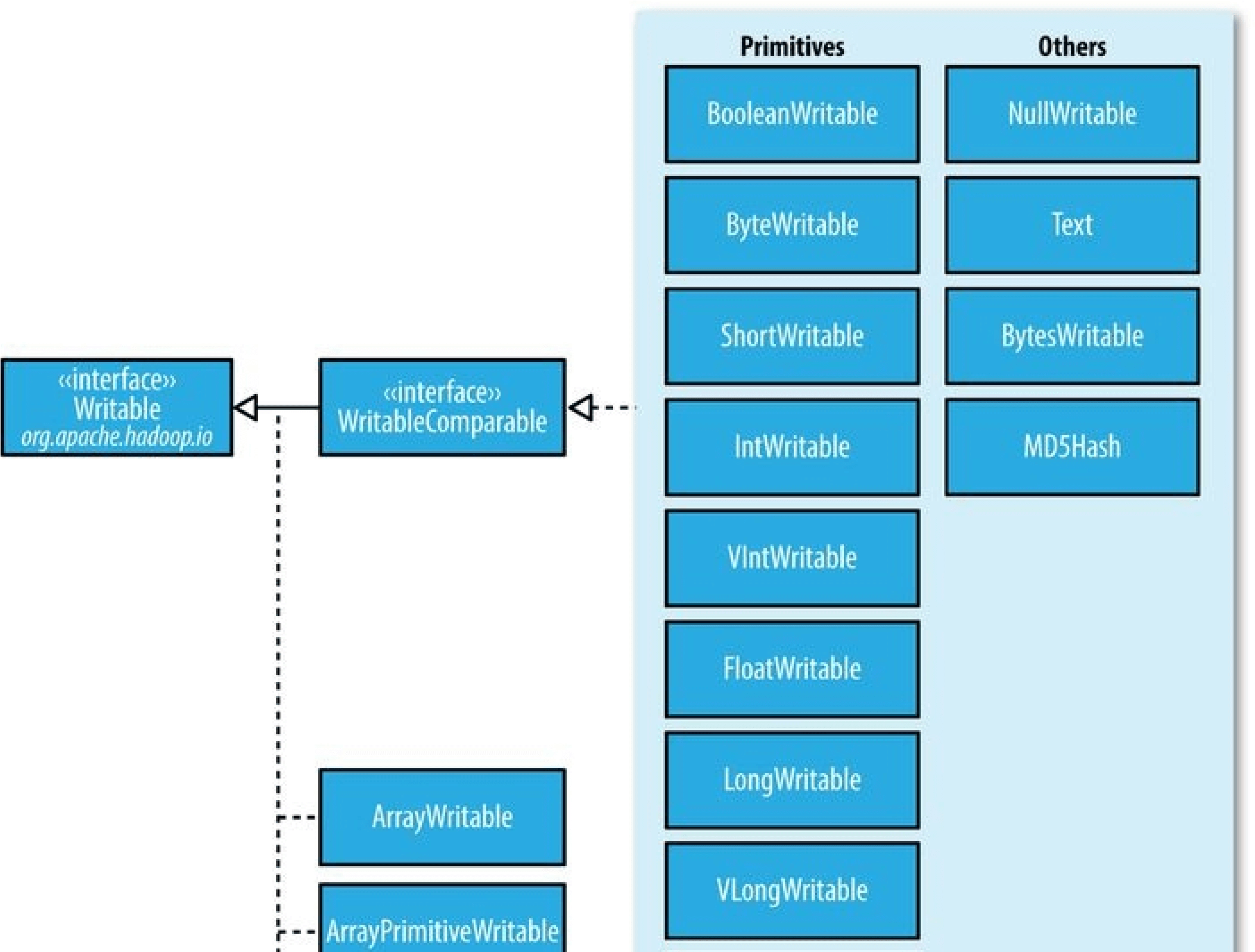
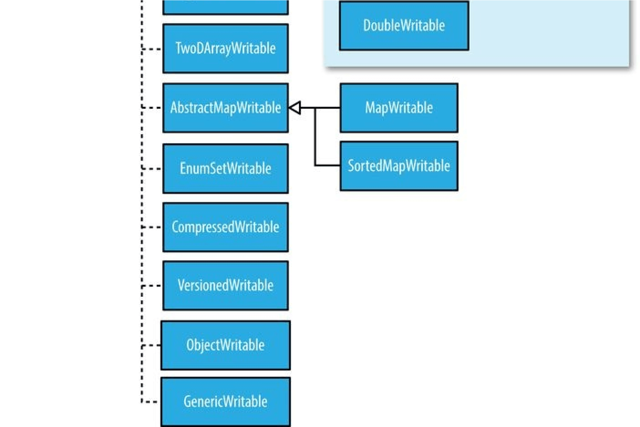
Figure 5-1. Writable class hierarchy
How do you choose between a fixed-length and a variable-length encoding? Fixed-length encodings are good when the distribution of values is fairly uniform across the whole value space, such as when using a (well-designed) hash function. Most numeric variables tend to have nonuniform distributions, though, and on average, the variable-length encoding will save space. Another advantage of variable-length encodings is that you can switch from VIntWritable to VLongWritable, because their encodings are actually the same. So, by choosing a variable-length representation, you have room to grow without committing to an 8-byte long representation from the beginning.
Text
Text is a Writable for UTF-8 sequences. It can be thought of as the Writable equivalent of java.lang.String.
The Text class uses an int (with a variable-length encoding) to store the number of bytes in the string encoding, so the maximum value is 2 GB. Furthermore, Text uses standard UTF-8, which makes it potentially easier to interoperate with other tools that understand UTF-8.
Indexing
Because of its emphasis on using standard UTF-8, there are some differences between
Text and the Java String class. Indexing for the Text class is in terms of position in the encoded byte sequence, not the Unicode character in the string or the Java char code unit (as it is for String). For ASCII strings, these three concepts of index position coincide. Here is an example to demonstrate the use of the charAt() method:
Text t = new Text(“hadoop”);
assertThat(t.getLength(), is(6)); assertThat(t.getBytes().length, is(6));
assertThat(t.charAt(2), is((int) ‘d’)); assertThat(“Out of bounds”, t.charAt(100), is(-1));
Notice that charAt() returns an int representing a Unicode code point, unlike the String variant that returns a char. Text also has a find() method, which is analogous to String’s indexOf():
Text t = new Text(“hadoop”);
assertThat(“Find a substring”, t.find(“do”), is(2)); assertThat(“Finds first ‘o’”, t.find(“o”), is(3)); assertThat(“Finds ‘o’ from position 4 or later”, t.find(“o”, 4), is(4)); assertThat(“No match”, t.find(“pig”), is(-1));
Unicode
When we start using characters that are encoded with more than a single byte, the differences between Text and String become clear. Consider the Unicode characters shown in Table 5-8.45]
Table 5-8. Unicode characters
| Unicode code point | U+0041 | U+00DF U+6771 | U+10400 |
|---|---|---|---|
| Name | LATIN CAPITAL LETTER A |
LATIN SMALL LETTER N/A (a unified Han SHARP S ideograph) |
DESERET CAPITAL LETTER LONG I |
| UTF-8 code units | 41 | c3 9f e6 9d b1 | f0 90 90 80 |
| Java \u0041 representation |
\u00DF \u6771 | \uD801\uDC00 |
All but the last character in the table, U+10400, can be expressed using a single Java char. U+10400 is a supplementary character and is represented by two Java chars, known as a surrogate pair. The tests in Example 5-5 show the differences between String and Text when processing a string of the four characters from Table 5-8.
Example 5-5. Tests showing the differences between the String and Text classes
public class StringTextComparisonTest {
@Test
public void string() throws UnsupportedEncodingException {
String s = “\u0041\u00DF\u6771\uD801\uDC00”; assertThat(s.length(), is(5)); assertThat(s.getBytes(“UTF-8”).length, is(10));
assertThat(s.indexOf(“\u0041”), is(0)); assertThat(s.indexOf(“\u00DF”), is(1)); assertThat(s.indexOf(“\u6771”), is(2)); assertThat(s.indexOf(“\uD801\uDC00”), is(3));
assertThat(s.charAt(0), is(‘\u0041’)); assertThat(s.charAt(1), is(‘\u00DF’)); assertThat(s.charAt(2), is(‘\u6771’)); assertThat(s.charAt(3), is(‘\uD801’)); assertThat(s.charAt(4), is(‘\uDC00’));
assertThat(s.codePointAt(0), is(0x0041)); assertThat(s.codePointAt(1), is(0x00DF)); assertThat(s.codePointAt(2), is(0x6771)); assertThat(s.codePointAt(3), is(0x10400)); }
@Test
public void text() {
Text t = new Text(“\u0041\u00DF\u6771\uD801\uDC00”); assertThat(t.getLength(), is(10));
assertThat(t.find(“\u0041”), is(0)); assertThat(t.find(“\u00DF”), is(1)); assertThat(t.find(“\u6771”), is(3)); assertThat(t.find(“\uD801\uDC00”), is(6));
assertThat(t.charAt(0), is(0x0041)); assertThat(t.charAt(1), is(0x00DF)); assertThat(t.charAt(3), is(0x6771)); assertThat(t.charAt(6), is(0x10400));
} }
The test confirms that the length of a String is the number of char code units it contains (five, made up of one from each of the first three characters in the string and a surrogate pair from the last), whereas the length of a Text object is the number of bytes in its UTF-8 encoding (10 = 1+2+3+4). Similarly, the indexOf() method in String returns an index in char code units, and find() for Text returns a byte offset.
The charAt() method in String returns the char code unit for the given index, which in the case of a surrogate pair will not represent a whole Unicode character. The codePointAt() method, indexed by char code unit, is needed to retrieve a single Unicode character represented as an int. In fact, the charAt() method in Text is more like the codePointAt() method than its namesake in String. The only difference is that it is indexed by byte offset.
Iteration
Iterating over the Unicode characters in Text is complicated by the use of byte offsets for indexing, since you can’t just increment the index. The idiom for iteration is a little obscure (see Example 5-6): turn the Text object into a java.nio.ByteBuffer, then repeatedly call the bytesToCodePoint() static method on Text with the buffer. This method extracts the next code point as an int and updates the position in the buffer. The end of the string is detected when bytesToCodePoint() returns –1. Example 5-6. Iterating over the characters in a Text object
public class TextIterator {
public static void main(String[] args) {
Text t = new Text(“\u0041\u00DF\u6771\uD801\uDC00”);
ByteBuffer buf = ByteBuffer.wrap(t.getBytes(), 0, t.getLength()); int cp; while (buf.hasRemaining() && (cp = Text.bytesToCodePoint(buf)) != -1) {
System.out.println(Integer.toHexString(cp));
} } }
Running the program prints the code points for the four characters in the string:
% hadoop TextIterator
41 df 6771 10400
Mutability
Another difference from String is that Text is mutable (like all Writable implementations in Hadoop, except NullWritable, which is a singleton). You can reuse a Text instance by calling one of the set() methods on it. For example:
Text t = new Text(“hadoop”);
t.set(“pig”);
Resorting to String
Text doesn’t have as rich an API for manipulating strings as java.lang.String, so in many cases, you need to convert the Text object to a String. This is done in the usual way, using the toString() method: assertThat(new Text(“hadoop”).toString(), is(“hadoop”));
BytesWritable
BytesWritable is a wrapper for an array of binary data. Its serialized format is a 4-byte integer field that specifies the number of bytes to follow, followed by the bytes themselves. For example, the byte array of length 2 with values 3 and 5 is serialized as a 4-byte integer (00000002) followed by the two bytes from the array (03 and 05):
BytesWritable b = new BytesWritable(new byte[] { 3, 5 }); byte[] bytes = serialize(b); assertThat(StringUtils.byteToHexString(bytes), is(“000000020305”));
BytesWritable is mutable, and its value may be changed by calling its set() method. As with Text, the size of the byte array returned from the getBytes() method for
BytesWritable — the capacity — may not reflect the actual size of the data stored in the BytesWritable. You can determine the size of the BytesWritable by calling getLength(). To demonstrate:
b.setCapacity(11); assertThat(b.getLength(), is(2)); assertThat(b.getBytes().length, is(11));
NullWritable
NullWritable is a special type of Writable, as it has a zero-length serialization. No bytes are written to or read from the stream. It is used as a placeholder; for example, in MapReduce, a key or a value can be declared as a NullWritable when you don’t need to use that position, effectively storing a constant empty value. NullWritable can also be useful as a key in a SequenceFile when you want to store a list of values, as opposed to key-value pairs. It is an immutable singleton, and the instance can be retrieved by calling NullWritable.get().
ObjectWritable and GenericWritable
ObjectWritable is a general-purpose wrapper for the following: Java primitives, String, enum, Writable, null, or arrays of any of these types. It is used in Hadoop RPC to marshal and unmarshal method arguments and return types.
ObjectWritable is useful when a field can be of more than one type. For example, if the values in a SequenceFile have multiple types, you can declare the value type as an ObjectWritable and wrap each type in an ObjectWritable. Being a general-purpose mechanism, it wastes a fair amount of space because it writes the classname of the wrapped type every time it is serialized. In cases where the number of types is small and known ahead of time, this can be improved by having a static array of types and using the index into the array as the serialized reference to the type. This is the approach that
GenericWritable takes, and you have to subclass it to specify which types to support.
Writable collections
The org.apache.hadoop.io package includes six Writable collection types: ArrayWritable, ArrayPrimitiveWritable, TwoDArrayWritable, MapWritable, SortedMapWritable, and EnumSetWritable.
ArrayWritable and TwoDArrayWritable are Writable implementations for arrays and two-dimensional arrays (array of arrays) of Writable instances. All the elements of an ArrayWritable or a TwoDArrayWritable must be instances of the same class, which is specified at construction as follows:
ArrayWritable writable = new ArrayWritable(Text.class);
In contexts where the Writable is defined by type, such as in SequenceFile keys or values or as input to MapReduce in general, you need to subclass ArrayWritable (or TwoDArrayWritable, as appropriate) to set the type statically. For example:
public class TextArrayWritable extends ArrayWritable { public TextArrayWritable() { super(Text.class);
} }
ArrayWritable and TwoDArrayWritable both have get() and set() methods, as well as a toArray() method, which creates a shallow copy of the array (or 2D array).
ArrayPrimitiveWritable is a wrapper for arrays of Java primitives. The component type is detected when you call set(), so there is no need to subclass to set the type.
MapWritable is an implementation of java.util.Map
java.util.SortedMap
value field is a part of the serialization format for that field. The type is stored as a single byte that acts as an index into an array of types. The array is populated with the standard types in the org.apache.hadoop.io package, but custom Writable types are accommodated, too, by writing a header that encodes the type array for nonstandard types.
As they are implemented, MapWritable and SortedMapWritable use positive byte values for custom types, so a maximum of 127 distinct nonstandard Writable classes can be used in any particular MapWritable or SortedMapWritable instance. Here’s a demonstration of using a MapWritable with different types for keys and values:
MapWritable src = new MapWritable(); src.put(new IntWritable(1), new Text(“cat”)); src.put(new VIntWritable(2), new LongWritable(163));
MapWritable dest = new MapWritable(); WritableUtils.cloneInto(dest, src);
assertThat((Text) dest.get(new IntWritable(1)), is(new Text(“cat”))); assertThat((LongWritable) dest.get(new VIntWritable(2)), is(new LongWritable(163)));
Conspicuous by their absence are Writable collection implementations for sets and lists. A general set can be emulated by using a MapWritable (or a SortedMapWritable for a sorted set) with NullWritable values. There is also EnumSetWritable for sets of enum types. For lists of a single type of Writable, ArrayWritable is adequate, but to store different types of Writable in a single list, you can use GenericWritable to wrap the elements in an ArrayWritable. Alternatively, you could write a general ListWritable using the ideas from MapWritable.
Implementing a Custom Writable
Hadoop comes with a useful set of Writable implementations that serve most purposes; however, on occasion, you may need to write your own custom implementation. With a custom Writable, you have full control over the binary representation and the sort order. Because Writables are at the heart of the MapReduce data path, tuning the binary representation can have a significant effect on performance. The stock Writable implementations that come with Hadoop are well tuned, but for more elaborate structures, it is often better to create a new Writable type rather than composing the stock types.
TIP
If you are considering writing a custom Writable, it may be worth trying another serialization framework, like Avro, that allows you to define custom types declaratively. See Serialization Frameworks and Chapter 12.
To demonstrate how to create a custom Writable, we shall write an implementation that represents a pair of strings, called TextPair. The basic implementation is shown in Example 5-7.
Example 5-7. A Writable implementation that stores a pair of Text objects
import java.io.*; import org.apache.hadoop.io.*; public class TextPair implements WritableComparable
private Text first; private Text second;
public TextPair() {
set(new Text(), new Text());
}
public TextPair(String first, String second) { set(new Text(first), new Text(second)); }
public TextPair(Text first, Text second) { set(first, second);
}
public void set(Text first, Text second) { this.first = first; this.second = second; }
public Text getFirst() { return first;
}
public Text getSecond() { return second; }
@Override
public void write(DataOutput out) throws IOException { first.write(out); second.write(out); }
@Override
public void readFields(DataInput in) throws IOException { first.readFields(in); second.readFields(in);
}
@Override
public int hashCode() { return first.hashCode() 163 + second.hashCode();
}
@Override
public boolean equals(Object o) { if (o instanceof TextPair) { TextPair tp = (TextPair) o;
return first.equals(tp.first) && second.equals(tp.second);
}
return false; }
@Override
public String toString() { return first + “\t” + second;
}
@Override
public int compareTo(TextPair tp) { int cmp = first.compareTo(tp.first); if (cmp != 0) { return cmp;
}
return second.compareTo(tp.second);
} }
The first part of the implementation is straightforward: there are two Text instance variables, first and second, and associated constructors, getters, and setters. All Writable implementations must have a default constructor so that the MapReduce framework can instantiate them, then populate their fields by calling readFields(). Writable instances are mutable and often reused, so you should take care to avoid allocating objects in the write() or readFields() methods.
TextPair’s write() method serializes each Text object in turn to the output stream by delegating to the Text objects themselves. Similarly, readFields() deserializes the bytes from the input stream by delegating to each Text object. The DataOutput and DataInput interfaces have a rich set of methods for serializing and deserializing Java primitives, so, in general, you have complete control over the wire format of your Writable object.
Just as you would for any value object you write in Java, you should override the hashCode(), equals(), and toString() methods from java.lang.Object. The hashCode() method is used by the HashPartitioner (the default partitioner in
MapReduce) to choose a reduce partition, so you should make sure that you write a good hash function that mixes well to ensure reduce partitions are of a similar size.
*WARNING
If you plan to use your custom Writable with TextOutputFormat, you must implement its toString() method. TextOutputFormat calls toString() on keys and values for their output representation. For TextPair, we write the underlying Text objects as strings separated by a tab character.
TextPair is an implementation of WritableComparable, so it provides an implementation of the compareTo() method that imposes the ordering you would expect: it sorts by the first string followed by the second. Notice that, apart from the number of Text objects it can store, TextPair differs from TextArrayWritable (which we discussed in the previous section), since TextArrayWritable is only a Writable, not a WritableComparable.
Implementing a RawComparator for speed
The code for TextPair in Example 5-7 will work as it stands; however, there is a further optimization we can make. As explained in WritableComparable and comparators, when TextPair is being used as a key in MapReduce, it will have to be deserialized into an object for the compareTo() method to be invoked. What if it were possible to compare two TextPair objects just by looking at their serialized representations?
It turns out that we can do this because TextPair is the concatenation of two Text objects, and the binary representation of a Text object is a variable-length integer containing the number of bytes in the UTF-8 representation of the string, followed by the UTF-8 bytes themselves. The trick is to read the initial length so we know how long the first Text object’s byte representation is; then we can delegate to Text’s RawComparator and invoke it with the appropriate offsets for the first or second string. Example 5-8 gives the details (note that this code is nested in the TextPair class).
Example 5-8. A RawComparator for comparing TextPair byte representations
public static class Comparator extends WritableComparator {
private static final Text.Comparator TEXT_COMPARATOR = new Text.Comparator();
public Comparator() { super(TextPair.class); }
@Override
public int compare(byte[] b1, int s1, int l1, byte[] b2, int s2, int l2) {
try { int firstL1 = WritableUtils.decodeVIntSize(b1[s1]) + readVInt(b1, s1); int firstL2 = WritableUtils.decodeVIntSize(b2[s2]) + readVInt(b2, s2); int cmp = TEXT_COMPARATOR.compare(b1, s1, firstL1, b2, s2, firstL2); if (cmp != 0) { return cmp;
}
return TEXT_COMPARATOR.compare(b1, s1 + firstL1, l1 - firstL1, b2, s2 + firstL2, l2 - firstL2);
} catch (IOException e) {
throw new IllegalArgumentException(e); }
} }
static {
WritableComparator.define(TextPair.class, new Comparator()); }
We actually subclass WritableComparator rather than implementing RawComparator directly, since it provides some convenience methods and default implementations. The subtle part of this code is calculating firstL1 and firstL2, the lengths of the first Text field in each byte stream. Each is made up of the length of the variable-length integer (returned by decodeVIntSize() on WritableUtils) and the value it is encoding (returned by readVInt()).
The static block registers the raw comparator so that whenever MapReduce sees the TextPair class, it knows to use the raw comparator as its default comparator.
Custom comparators
As you can see with TextPair, writing raw comparators takes some care because you have to deal with details at the byte level. It is worth looking at some of the implementations of Writable in the org.apache.hadoop.io package for further ideas if you need to write your own. The utility methods on WritableUtils are very handy, too.
Custom comparators should also be written to be RawComparators, if possible. These are comparators that implement a different sort order from the natural sort order defined by the default comparator. Example 5-9 shows a comparator for TextPair, called
FirstComparator, that considers only the first string of the pair. Note that we override the compare() method that takes objects so both compare() methods have the same semantics.
We will make use of this comparator in Chapter 9, when we look at joins and secondary sorting in MapReduce (see Joins).
Example 5-9. A custom RawComparator for comparing the first field of TextPair byte representations
public static class FirstComparator extends WritableComparator {
private static final Text.Comparator TEXT_COMPARATOR = new Text.Comparator();
public FirstComparator() { super(TextPair.class); }
@Override
public int compare(byte[] b1, int s1, int l1, byte[] b2, int s2, int l2) {
try { int firstL1 = WritableUtils.decodeVIntSize(b1[s1]) + readVInt(b1, s1); int firstL2 = WritableUtils.decodeVIntSize(b2[s2]) + readVInt(b2, s2); return TEXT_COMPARATOR.compare(b1, s1, firstL1, b2, s2, firstL2);
} catch (IOException e) {
throw new IllegalArgumentException(e);
}
}
@Override
public int compare(WritableComparable a, WritableComparable b) { if (a instanceof TextPair && b instanceof TextPair) {
return ((TextPair) a).first.compareTo(((TextPair) b).first);
}
return super.compare(a, b);
} }
Serialization Frameworks
Although most MapReduce programs use Writable key and value types, this isn’t mandated by the MapReduce API. In fact, any type can be used; the only requirement is a mechanism that translates to and from a binary representation of each type.
To support this, Hadoop has an API for pluggable serialization frameworks. A serialization framework is represented by an implementation of Serialization (in the org.apache.hadoop.io.serializer package). WritableSerialization, for example, is the implementation of Serialization for Writable types.
A Serialization defines a mapping from types to Serializer instances (for turning an object into a byte stream) and Deserializer instances (for turning a byte stream into an object).
Set the io.serializations property to a comma-separated list of classnames in order to register Serialization implementations. Its default value includes
org.apache.hadoop.io.serializer.WritableSerialization and the Avro Specific and Reflect serializations (see Avro Data Types and Schemas), which means that only Writable or Avro objects can be serialized or deserialized out of the box.
Hadoop includes a class called JavaSerialization that uses Java Object Serialization.
Although it makes it convenient to be able to use standard Java types such as Integer or String in MapReduce programs, Java Object Serialization is not as efficient as Writables, so it’s not worth making this trade-off (see the following sidebar).
WHY NOT USE JAVA OBJECT SERIALIZATION?
Java comes with its own serialization mechanism, called Java Object Serialization (often referred to simply as “Java Serialization”), that is tightly integrated with the language, so it’s natural to ask why this wasn’t used in Hadoop. Here’s what Doug Cutting said in response to that question:
Why didn’t I use Serialization when we first started Hadoop? Because it looked big and hairy and I thought we needed something lean and mean, where we had precise control over exactly how objects are written and read, since that is central to Hadoop. With Serialization you can get some control, but you have to fight for it.
The logic for not using RMI [Remote Method Invocation] was similar. Effective, high-performance inter-process communications are critical to Hadoop. I felt like we’d need to precisely control how things like connections, timeouts and buffers are handled, and RMI gives you little control over those.
The problem is that Java Serialization doesn’t meet the criteria for a serialization format listed earlier: compact, fast, extensible, and interoperable.
Serialization IDL
There are a number of other serialization frameworks that approach the problem in a different way: rather than defining types through code, you define them in a languageneutral, declarative fashion, using an interface description language (IDL). The system can then generate types for different languages, which is good for interoperability. They also typically define versioning schemes that make type evolution straightforward.
Apache Thrift and Google Protocol Buffers are both popular serialization frameworks, and both are commonly used as a format for persistent binary data. There is limited support for these as MapReduce formats;46] however, they are used internally in parts of Hadoop for RPC and data exchange.
Avro is an IDL-based serialization framework designed to work well with large-scale data processing in Hadoop. It is covered in Chapter 12.
File-Based Data Structures
For some applications, you need a specialized data structure to hold your data. For doing MapReduce-based processing, putting each blob of binary data into its own file doesn’t scale, so Hadoop developed a number of higher-level containers for these situations.
SequenceFile
Imagine a logfile where each log record is a new line of text. If you want to log binary types, plain text isn’t a suitable format. Hadoop’s SequenceFile class fits the bill in this situation, providing a persistent data structure for binary key-value pairs. To use it as a logfile format, you would choose a key, such as timestamp represented by a
LongWritable, and the value would be a Writable that represents the quantity being logged.
SequenceFiles also work well as containers for smaller files. HDFS and MapReduce are optimized for large files, so packing files into a SequenceFile makes storing and processing the smaller files more efficient (Processing a whole file as a record contains a program to pack files into a SequenceFile).47]
Writing a SequenceFile
To create a SequenceFile, use one of its createWriter() static methods, which return a SequenceFile.Writer instance. There are several overloaded versions, but they all require you to specify a stream to write to (either an FSDataOutputStream or a FileSystem and Path pairing), a Configuration object, and the key and value types. Optional arguments include the compression type and codec, a Progressable callback to be informed of write progress, and a Metadata instance to be stored in the SequenceFile header.
The keys and values stored in a SequenceFile do not necessarily need to be Writables. Any types that can be serialized and deserialized by a Serialization may be used.
Once you have a SequenceFile.Writer, you then write key-value pairs using the append() method. When you’ve finished, you call the close() method (SequenceFile.Writer implements java.io.Closeable).
Example 5-10 shows a short program to write some key-value pairs to a SequenceFile using the API just described.
Example 5-10. Writing a SequenceFile
public class SequenceFileWriteDemo {
private static final String[] DATA = {
“One, two, buckle my shoe”,
“Three, four, shut the door”,
“Five, six, pick up sticks”,
“Seven, eight, lay them straight”,
“Nine, ten, a big fat hen”
};
public static void main(String[] args) throws IOException {
String uri = args[0];
Configuration conf = new Configuration();
FileSystem fs = FileSystem.get(URI.create(uri), conf); Path path = new Path(uri);
IntWritable key = new IntWritable();
Text value = new Text();
SequenceFile.Writer writer = null; try { writer = SequenceFile.createWriter(fs, conf, path, key.getClass(), value.getClass());
for (int i = 0; i < 100; i++) { key.set(100 - i); value.set(DATA[i % DATA.length]);
System.out.printf(“[%s]\t%s\t%s\n”, writer.getLength(), key, value); writer.append(key, value);
}
} finally {
IOUtils.closeStream(writer);
}
} }
The keys in the sequence file are integers counting down from 100 to 1, represented as
IntWritable objects. The values are Text objects. Before each record is appended to the SequenceFile.Writer, we call the getLength() method to discover the current position in the file. (We will use this information about record boundaries in the next section, when we read the file nonsequentially.) We write the position out to the console, along with the key and value pairs. The result of running it is shown here:
% hadoop SequenceFileWriteDemo numbers.seq
[128] 100 One, two, buckle my shoe
[173] 99 Three, four, shut the door
[220] 98 Five, six, pick up sticks
[264] 97 Seven, eight, lay them straight
[314] 96 Nine, ten, a big fat hen
[359] 95 One, two, buckle my shoe
[404] 94 Three, four, shut the door
[451] 93 Five, six, pick up sticks
[495] 92 Seven, eight, lay them straight
[545] 91 Nine, ten, a big fat hen…
[1976] 60 One, two, buckle my shoe
[2021] 59 Three, four, shut the door
[2088] 58 Five, six, pick up sticks
[2132] 57 Seven, eight, lay them straight
[2182] 56 Nine, ten, a big fat hen…
[4557] 5 One, two, buckle my shoe
[4602] 4 Three, four, shut the door
[4649] 3 Five, six, pick up sticks
[4693] 2 Seven, eight, lay them straight
[4743] 1 Nine, ten, a big fat hen
Reading a SequenceFile
Reading sequence files from beginning to end is a matter of creating an instance of
SequenceFile.Reader and iterating over records by repeatedly invoking one of the next() methods. Which one you use depends on the serialization framework you are using. If you are using Writable types, you can use the next() method that takes a key and a value argument and reads the next key and value in the stream into these variables: public boolean next(Writable key, Writable val)
The return value is true if a key-value pair was read and false if the end of the file has been reached.
For other, non-Writable serialization frameworks (such as Apache Thrift), you should use these two methods:
public Object next(Object key) throws IOException public Object getCurrentValue(Object val) throws IOException
In this case, you need to make sure that the serialization you want to use has been set in the io.serializations property; see Serialization Frameworks.
If the next() method returns a non-null object, a key-value pair was read from the stream, and the value can be retrieved using the getCurrentValue() method. Otherwise, if next() returns null, the end of the file has been reached.
The program in Example 5-11 demonstrates how to read a sequence file that has Writable keys and values. Note how the types are discovered from the SequenceFile.Reader via calls to getKeyClass() and getValueClass(), and then ReflectionUtils is used to create an instance for the key and an instance for the value. This technique allows the program to be used with any sequence file that has Writable keys and values. Example 5-11. Reading a SequenceFile
public class SequenceFileReadDemo {
public static void main(String[] args) throws IOException {
String uri = args[0];
Configuration conf = new Configuration();
FileSystem fs = FileSystem.get(URI.create(uri), conf);
Path path = new Path(uri);
SequenceFile.Reader reader = null; try { reader = new SequenceFile.Reader(fs, path, conf);
Writable key = (Writable)
ReflectionUtils.newInstance(reader.getKeyClass(), conf);
Writable value = (Writable)
ReflectionUtils.newInstance(reader.getValueClass(), conf); long position = reader.getPosition(); while (reader.next(key, value)) {
String syncSeen = reader.syncSeen() ? ““ : “”;
System.out.printf(“[%s%s]\t%s\t%s\n”, position, syncSeen, key, value); position = reader.getPosition(); // beginning of next record
}
} finally {
IOUtils.closeStream(reader);
}
} }
Another feature of the program is that it displays the positions of the sync points in the sequence file. A sync point is a point in the stream that can be used to resynchronize with a record boundary if the reader is “lost” — for example, after seeking to an arbitrary position in the stream. Sync points are recorded by SequenceFile.Writer, which inserts a special entry to mark the sync point every few records as a sequence file is being written.
Such entries are small enough to incur only a modest storage overhead — less than 1%. Sync points always align with record boundaries.
Running the program in Example 5-11 shows the sync points in the sequence file as asterisks. The first one occurs at position 2021 (the second one occurs at position 4075, but is not shown in the output):
% hadoop SequenceFileReadDemo numbers.seq
[128] 100 One, two, buckle my shoe
[173] 99 Three, four, shut the door
[220] 98 Five, six, pick up sticks
[264] 97 Seven, eight, lay them straight
[314] 96 Nine, ten, a big fat hen
[359] 95 One, two, buckle my shoe
[404] 94 Three, four, shut the door
[451] 93 Five, six, pick up sticks
[495] 92 Seven, eight, lay them straight
[545] 91 Nine, ten, a big fat hen
[590] 90 One, two, buckle my shoe…
[1976] 60 One, two, buckle my shoe
[2021] 59 Three, four, shut the door
[2088] 58 Five, six, pick up sticks
[2132] 57 Seven, eight, lay them straight
[2182] 56 Nine, ten, a big fat hen…
[4557] 5 One, two, buckle my shoe
[4602] 4 Three, four, shut the door
[4649] 3 Five, six, pick up sticks
[4693] 2 Seven, eight, lay them straight
[4743] 1 Nine, ten, a big fat hen
There are two ways to seek to a given position in a sequence file. The first is the seek() method, which positions the reader at the given point in the file. For example, seeking to a record boundary works as expected:
reader.seek(359); assertThat(reader.next(key, value), is(true)); assertThat(((IntWritable) key).get(), is(95));
But if the position in the file is not at a record boundary, the reader fails when the next() method is called:
reader.seek(360); reader.next(key, value); // fails with IOException
The second way to find a record boundary makes use of sync points. The sync(long position) method on SequenceFile.Reader positions the reader at the next sync point after position. (If there are no sync points in the file after this position, then the reader will be positioned at the end of the file.) Thus, we can call sync() with any position in the stream — not necessarily a record boundary — and the reader will reestablish itself at the next sync point so reading can continue:
reader.sync(360); assertThat(reader.getPosition(), is(2021L)); assertThat(reader.next(key, value), is(true)); assertThat(((IntWritable) key).get(), is(59));
WARNING
SequenceFile.Writer has a method called sync() for inserting a sync point at the current position in the stream. This is not to be confused with the hsync() method defined by the Syncable interface for synchronizing buffers to the underlying device (see Coherency Model).
Sync points come into their own when using sequence files as input to MapReduce, since they permit the files to be split and different portions to be processed independently by separate map tasks (see SequenceFileInputFormat).
Displaying a SequenceFile with the command-line interface
The hadoop fs command has a -text option to display sequence files in textual form. It looks at a file’s magic number so that it can attempt to detect the type of the file and appropriately convert it to text. It can recognize gzipped files, sequence files, and Avro datafiles; otherwise, it assumes the input is plain text.
For sequence files, this command is really useful only if the keys and values have meaningful string representations (as defined by the toString() method). Also, if you have your own key or value classes, you will need to make sure they are on Hadoop’s classpath.
Running it on the sequence file we created in the previous section gives the following output:
% hadoop fs -text numbers.seq | head
100 One, two, buckle my shoe
99 Three, four, shut the door
98 Five, six, pick up sticks
97 Seven, eight, lay them straight
96 Nine, ten, a big fat hen
95 One, two, buckle my shoe
94 Three, four, shut the door
93 Five, six, pick up sticks
92 Seven, eight, lay them straight
91 Nine, ten, a big fat hen
Sorting and merging SequenceFiles
The most powerful way of sorting (and merging) one or more sequence files is to use MapReduce. MapReduce is inherently parallel and will let you specify the number of reducers to use, which determines the number of output partitions. For example, by specifying one reducer, you get a single output file. We can use the sort example that comes with Hadoop by specifying that the input and output are sequence files and by setting the key and value types:
% hadoop jar \
$HADOOP_HOME/share/hadoop/mapreduce/hadoop-mapreduce-examples-*.jar \ sort -r 1 \
-inFormat org.apache.hadoop.mapreduce.lib.input.SequenceFileInputFormat \ -outFormat org.apache.hadoop.mapreduce.lib.output.SequenceFileOutputFormat \
-outKey org.apache.hadoop.io.IntWritable \ -outValue org.apache.hadoop.io.Text \ numbers.seq sorted
% hadoop fs -text sorted/part-r-00000 | head
1 Nine, ten, a big fat hen
2 Seven, eight, lay them straight
3 Five, six, pick up sticks
4 Three, four, shut the door
5 One, two, buckle my shoe
6 Nine, ten, a big fat hen
7 Seven, eight, lay them straight
8 Five, six, pick up sticks
9 Three, four, shut the door
10 One, two, buckle my shoe
Sorting is covered in more detail in Sorting.
An alternative to using MapReduce for sort/merge is the SequenceFile.Sorter class, which has a number of sort() and merge() methods. These functions predate MapReduce and are lower-level functions than MapReduce (for example, to get parallelism, you need to partition your data manually), so in general MapReduce is the preferred approach to sort and merge sequence files.
The SequenceFile format
A sequence file consists of a header followed by one or more records (see Figure 5-2). The first three bytes of a sequence file are the bytes SEQ, which act as a magic number; these are followed by a single byte representing the version number. The header contains other fields, including the names of the key and value classes, compression details, user-defined metadata, and the sync marker.48] Recall that the sync marker is used to allow a reader to synchronize to a record boundary from any position in the file. Each file has a randomly generated sync marker, whose value is stored in the header. Sync markers appear between records in the sequence file. They are designed to incur less than a 1% storage overhead, so they don’t necessarily appear between every pair of records (such is the case for short records).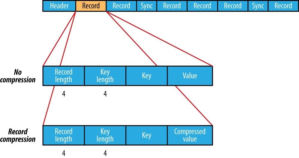
Figure 5-2. The internal structure of a sequence file with no compression and with record compression
The internal format of the records depends on whether compression is enabled, and if it is, whether it is record compression or block compression.
If no compression is enabled (the default), each record is made up of the record length (in bytes), the key length, the key, and then the value. The length fields are written as 4-byte integers adhering to the contract of the writeInt() method of java.io.DataOutput. Keys and values are serialized using the Serialization defined for the class being written to the sequence file.
The format for record compression is almost identical to that for no compression, except the value bytes are compressed using the codec defined in the header. Note that keys are not compressed.
Block compression (Figure 5-3) compresses multiple records at once; it is therefore more compact than and should generally be preferred over record compression because it has the opportunity to take advantage of similarities between records. Records are added to a block until it reaches a minimum size in bytes, defined by the io.seqfile.compress.blocksize property; the default is one million bytes. A sync marker is written before the start of every block. The format of a block is a field indicating the number of records in the block, followed by four compressed fields: the key lengths, the keys, the value lengths, and the values.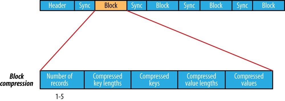
Figure 5-3. The internal structure of a sequence file with block compression
MapFile
A MapFile is a sorted SequenceFile with an index to permit lookups by key. The index is itself a SequenceFile that contains a fraction of the keys in the map (every 128th key, by default). The idea is that the index can be loaded into memory to provide fast lookups from the main data file, which is another SequenceFile containing all the map entries in sorted key order.
MapFile offers a very similar interface to SequenceFile for reading and writing — the main thing to be aware of is that when writing using MapFile.Writer, map entries must be added in order, otherwise an IOException will be thrown.
MapFile variants
Hadoop comes with a few variants on the general key-value MapFile interface:
SetFile is a specialization of MapFile for storing a set of Writable keys. The keys must be added in sorted order.
ArrayFile is a MapFile where the key is an integer representing the index of the element in the array and the value is a Writable value.
BloomMapFile is a MapFile that offers a fast version of the get() method, especially for sparsely populated files. The implementation uses a dynamic Bloom filter for testing whether a given key is in the map. The test is very fast because it is in-memory, and it has a nonzero probability of false positives. Only if the test passes (the key is present) is the regular get() method called.
Other File Formats and Column-Oriented Formats
While sequence files and map files are the oldest binary file formats in Hadoop, they are not the only ones, and in fact there are better alternatives that should be considered for new projects.
Avro datafiles (covered in Avro Datafiles) are like sequence files in that they are designed for large-scale data processing — they are compact and splittable — but they are portable across different programming languages. Objects stored in Avro datafiles are described by a schema, rather than in the Java code of the implementation of a Writable object (as is the case for sequence files), making them very Java-centric. Avro datafiles are widely supported across components in the Hadoop ecosystem, so they are a good default choice for a binary format.
Sequence files, map files, and Avro datafiles are all row-oriented file formats, which means that the values for each row are stored contiguously in the file. In a columnoriented format, the rows in a file (or, equivalently, a table in Hive) are broken up into row splits, then each split is stored in column-oriented fashion: the values for each row in the first column are stored first, followed by the values for each row in the second column, and so on. This is shown diagrammatically in Figure 5-4.
A column-oriented layout permits columns that are not accessed in a query to be skipped. Consider a query of the table in Figure 5-4 that processes only column 2. With roworiented storage, like a sequence file, the whole row (stored in a sequence file record) is loaded into memory, even though only the second column is actually read. Lazy deserialization saves some processing cycles by deserializing only the column fields that are accessed, but it can’t avoid the cost of reading each row’s bytes from disk.
With column-oriented storage, only the column 2 parts of the file (highlighted in the figure) need to be read into memory. In general, column-oriented formats work well when queries access only a small number of columns in the table. Conversely, row-oriented formats are appropriate when a large number of columns of a single row are needed for processing at the same time.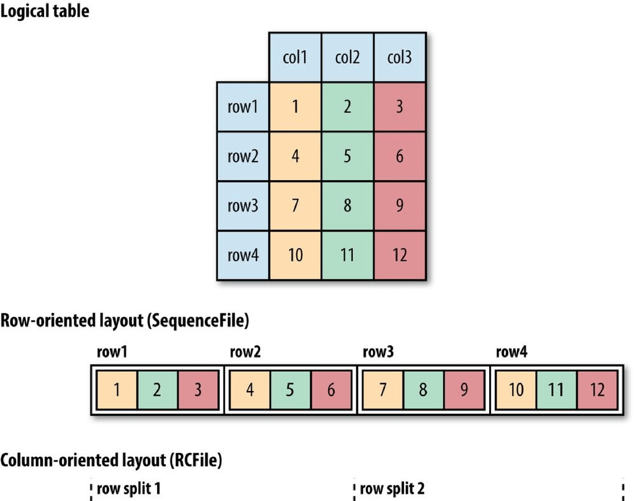
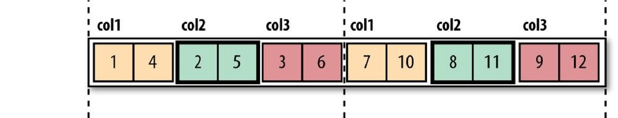
Figure 5-4. Row-oriented versus column-oriented storage
Column-oriented formats need more memory for reading and writing, since they have to buffer a row split in memory, rather than just a single row. Also, it’s not usually possible to control when writes occur (via flush or sync operations), so column-oriented formats are not suited to streaming writes, as the current file cannot be recovered if the writer process fails. On the other hand, row-oriented formats like sequence files and Avro datafiles can be read up to the last sync point after a writer failure. It is for this reason that Flume (see Chapter 14) uses row-oriented formats.
The first column-oriented file format in Hadoop was Hive’s RCFile, short for Record
Columnar File. It has since been superseded by Hive’s ORCFile (Optimized Record Columnar File), and Parquet (covered in Chapter 13). Parquet is a general-purpose column-oriented file format based on Google’s Dremel, and has wide support across Hadoop components. Avro also has a column-oriented format called Trevni.
[44] For a comprehensive set of compression benchmarks, jvm-compressor-benchmark is a good reference for JVMcompatible libraries (including some native libraries).
[45] This example is based on one from Norbert Lindenberg and Masayoshi Okutsu’s “Supplementary Characters in the Java Platform,” May 2004.
[46] Twitter’s Elephant Bird project includes tools for working with Thrift and Protocol Buffers in Hadoop.
[47] In a similar vein, the blog post “A Million Little Files” by Stuart Sierra includes code for converting a tar file into a SequenceFile.
[48] Full details of the format of these fields may be found in SequenceFile’s documentation and source code.
Part II. MapReduce
Chapter 6. Developing a MapReduce Application
In Chapter 2, we introduced the MapReduce model. In this chapter, we look at the practical aspects of developing a MapReduce application in Hadoop.
Writing a program in MapReduce follows a certain pattern. You start by writing your map and reduce functions, ideally with unit tests to make sure they do what you expect. Then you write a driver program to run a job, which can run from your IDE using a small subset of the data to check that it is working. If it fails, you can use your IDE’s debugger to find the source of the problem. With this information, you can expand your unit tests to cover this case and improve your mapper or reducer as appropriate to handle such input correctly.
When the program runs as expected against the small dataset, you are ready to unleash it on a cluster. Running against the full dataset is likely to expose some more issues, which you can fix as before, by expanding your tests and altering your mapper or reducer to handle the new cases. Debugging failing programs in the cluster is a challenge, so we’ll look at some common techniques to make it easier.
After the program is working, you may wish to do some tuning, first by running through some standard checks for making MapReduce programs faster and then by doing task profiling. Profiling distributed programs is not easy, but Hadoop has hooks to aid in the process.
Before we start writing a MapReduce program, however, we need to set up and configure the development environment. And to do that, we need to learn a bit about how Hadoop does configuration.
The Configuration API
Components in Hadoop are configured using Hadoop’s own configuration API. An instance of the Configuration class (found in the org.apache.hadoop.conf package) represents a collection of configuration properties and their values. Each property is named by a String, and the type of a value may be one of several, including Java primitives such as boolean, int, long, and float; other useful types such as String, Class, and java.io.File; and collections of Strings.
Configurations read their properties from resources — XML files with a simple structure for defining name-value pairs. See Example 6-1.
Example 6-1. A simple configuration file, configuration-1.xml
<?xml version=”1.0”?>
Assuming this Configuration is in a file called configuration-1.xml, we can access its properties using a piece of code like this:
Configuration conf = new Configuration(); conf.addResource(“configuration-1.xml”); assertThat(conf.get(“color”), is(“yellow”)); assertThat(conf.getInt(“size”, 0), is(10)); assertThat(conf.get(“breadth”, “wide”), is(“wide”));
There are a couple of things to note: type information is not stored in the XML file; instead, properties can be interpreted as a given type when they are read. Also, the get() methods allow you to specify a default value, which is used if the property is not defined in the XML file, as in the case of breadth here.
Combining Resources
Things get interesting when more than one resource is used to define a Configuration. This is used in Hadoop to separate out the default properties for the system, defined internally in a file called core-default.xml, from the site-specific overrides in core-site.xml. The file in Example 6-2 defines the size and weight properties.
Example 6-2. A second configuration file, configuration-2.xml
<?xml version=”1.0”?>
Resources are added to a Configuration in order:
Configuration conf = new Configuration(); conf.addResource(“configuration-1.xml”); conf.addResource(“configuration-2.xml”);
Properties defined in resources that are added later override the earlier definitions. So the size property takes its value from the second configuration file, configuration-2.xml: assertThat(conf.getInt(“size”, 0), is(12));
However, properties that are marked as final cannot be overridden in later definitions. The weight property is final in the first configuration file, so the attempt to override it in the second fails, and it takes the value from the first: assertThat(conf.get(“weight”), is(“heavy”));
Attempting to override final properties usually indicates a configuration error, so this results in a warning message being logged to aid diagnosis. Administrators mark properties as final in the daemon’s site files that they don’t want users to change in their client-side configuration files or job submission parameters.
Variable Expansion
Configuration properties can be defined in terms of other properties, or system properties.
For example, the property size-weight in the first configuration file is defined as ${size},${weight}, and these properties are expanded using the values found in the configuration: assertThat(conf.get(“size-weight”), is(“12,heavy”));
System properties take priority over properties defined in resource files:
System.setProperty(“size”, “14”); assertThat(conf.get(“size-weight”), is(“14,heavy”));
This feature is useful for overriding properties on the command line by using Dproperty=value JVM arguments.
Note that although configuration properties can be defined in terms of system properties, unless system properties are redefined using configuration properties, they are not accessible through the configuration API. Hence:
System.setProperty(“length”, “2”);
assertThat(conf.get(“length”), is((String) null));
Setting Up the Development Environment
The first step is to create a project so you can build MapReduce programs and run them in local (standalone) mode from the command line or within your IDE. The Maven Project Object Model (POM) in Example 6-3 shows the dependencies needed for building and testing MapReduce programs.
Example 6-3. A Maven POM for building and testing a MapReduce application
The dependencies section is the interesting part of the POM. (It is straightforward to use another build tool, such as Gradle or Ant with Ivy, as long as you use the same set of dependencies defined here.) For building MapReduce jobs, you only need to have the hadoop-client dependency, which contains all the Hadoop client-side classes needed to interact with HDFS and MapReduce. For running unit tests, we use junit, and for writing MapReduce tests, we use mrunit. The hadoop-minicluster library contains the “mini-” clusters that are useful for testing with Hadoop clusters running in a single JVM.
Many IDEs can read Maven POMs directly, so you can just point them at the directory containing the pom.xml file and start writing code. Alternatively, you can use Maven to generate configuration files for your IDE. For example, the following creates Eclipse configuration files so you can import the project into Eclipse:
% mvn eclipse:eclipse -DdownloadSources=true -DdownloadJavadocs=true
Managing Configuration
When developing Hadoop applications, it is common to switch between running the application locally and running it on a cluster. In fact, you may have several clusters you work with, or you may have a local “pseudodistributed” cluster that you like to test on (a pseudodistributed cluster is one whose daemons all run on the local machine; setting up this mode is covered in Appendix A).
One way to accommodate these variations is to have Hadoop configuration files containing the connection settings for each cluster you run against and specify which one you are using when you run Hadoop applications or tools. As a matter of best practice, it’s recommended to keep these files outside Hadoop’s installation directory tree, as this makes it easy to switch between Hadoop versions without duplicating or losing settings.
For the purposes of this book, we assume the existence of a directory called conf that contains three configuration files: hadoop-local.xml, hadoop-localhost.xml, and hadoopcluster.xml (these are available in the example code for this book). Note that there is nothing special about the names of these files; they are just convenient ways to package up some configuration settings. (Compare this to Table A-1 in Appendix A, which sets out the equivalent server-side configurations.)
The hadoop-local.xml file contains the default Hadoop configuration for the default filesystem and the local (in-JVM) framework for running MapReduce jobs:
<?xml version=”1.0”?>
The settings in hadoop-localhost.xml point to a namenode and a YARN resource manager both running on localhost:
<?xml version=”1.0”?>
Finally, hadoop-cluster.xml contains details of the cluster’s namenode and YARN resource manager addresses (in practice, you would name the file after the name of the cluster, rather than “cluster” as we have here):
<?xml version=”1.0”?>
You can add other configuration properties to these files as needed.
SETTING USER IDENTITY
The user identity that Hadoop uses for permissions in HDFS is determined by running the whoami command on the client system. Similarly, the group names are derived from the output of running groups.
If, however, your Hadoop user identity is different from the name of your user account on your client machine, you can explicitly set your Hadoop username by setting the HADOOPUSER_NAME environment variable. You can also override user group mappings by means of the hadoop.user.group.static.mapping.overrides configuration property. For example, dr.who=;preston=directors,inventors means that the dr.who user is in no groups, but preston is in the directors and inventors groups.
You can set the user identity that the Hadoop web interfaces run as by setting the hadoop.http.staticuser.user property. By default, it is dr.who, which is not a superuser, so system files are not accessible through the web interface.
Notice that, by default, there is no authentication with this system. See Security for how to use Kerberos authentication with Hadoop.
With this setup, it is easy to use any configuration with the -conf command-line switch. For example, the following command shows a directory listing on the HDFS server running in pseudodistributed mode on localhost:
% hadoop fs -conf conf/hadoop-localhost.xml -ls . Found 2 items
drwxr-xr-x - tom supergroup 0 2014-09-08 10:19 input drwxr-xr-x - tom supergroup 0 2014-09-08 10:19 output
If you omit the -conf option, you pick up the Hadoop configuration in the _etc/hadoop _subdirectory under $HADOOP_HOME. Or, if HADOOP_CONF_DIR is set, Hadoop configuration files will be read from that location.
NOTE
Here’s an alternative way of managing configuration settings. Copy the _etc/hadoop directory from your Hadoop installation to another location, place the *-site.xml configuration files there (with appropriate settings), and set the HADOOPCONF_DIR environment variable to the alternative location. The main advantage of this approach is that you don’t need to specify -conf for every command. It also allows you to isolate changes to files other than the Hadoop XML configuration files (e.g., _log4j.properties) since the HADOOP_CONF_DIR directory has a copy of all the configuration files (see Hadoop Configuration).
Tools that come with Hadoop support the -conf option, but it’s straightforward to make your programs (such as programs that run MapReduce jobs) support it, too, using the Tool interface.
GenericOptionsParser, Tool, and ToolRunner
Hadoop comes with a few helper classes for making it easier to run jobs from the command line. GenericOptionsParser is a class that interprets common Hadoop command-line options and sets them on a Configuration object for your application to use as desired. You don’t usually use GenericOptionsParser directly, as it’s more convenient to implement the Tool interface and run your application with the ToolRunner, which uses GenericOptionsParser internally:
public interface Tool extends Configurable { int run(String [] args) throws Exception; }
Example 6-4 shows a very simple implementation of Tool that prints the keys and values of all the properties in the Tool’s Configuration object.
Example 6-4. An example Tool implementation for printing the properties in a Configuration
public class ConfigurationPrinter extends Configured implements Tool {
static {
Configuration.addDefaultResource(“hdfs-default.xml”);
Configuration.addDefaultResource(“hdfs-site.xml”);
Configuration.addDefaultResource(“yarn-default.xml”);
Configuration.addDefaultResource(“yarn-site.xml”);
Configuration.addDefaultResource(“mapred-default.xml”); Configuration.addDefaultResource(“mapred-site.xml”); }
@Override
public int run(String[] args) throws Exception { Configuration conf = getConf();
for (Entry
System.out.printf(“%s=%s\n”, entry.getKey(), entry.getValue());
} return 0;
}
public static void main(String[] args) throws Exception {
int exitCode = ToolRunner.run(new ConfigurationPrinter(), args);
System.exit(exitCode);
} }
We make ConfigurationPrinter a subclass of Configured, which is an implementation of the Configurable interface. All implementations of Tool need to implement Configurable (since Tool extends it), and subclassing Configured is often the easiest way to achieve this. The run() method obtains the Configuration using Configurable’s getConf() method and then iterates over it, printing each property to standard output.
The static block makes sure that the HDFS, YARN, and MapReduce configurations are picked up, in addition to the core ones (which Configuration knows about already).
ConfigurationPrinter’s main() method does not invoke its own run() method directly.
Instead, we call ToolRunner’s static run() method, which takes care of creating a
Configuration object for the Tool before calling its run() method. ToolRunner also uses a GenericOptionsParser to pick up any standard options specified on the command line and to set them on the Configuration instance. We can see the effect of picking up the properties specified in conf/hadoop-localhost.xml by running the following commands:
% mvn compile
% export HADOOP_CLASSPATH=target/classes/
% hadoop ConfigurationPrinter -conf conf/hadoop-localhost.xml \
| grep yarn.resourcemanager.address= yarn.resourcemanager.address=localhost:8032
WHICH PROPERTIES CAN I SET?
ConfigurationPrinter is a useful tool for discovering what a property is set to in your environment. For a running daemon, like the namenode, you can see its configuration by viewing the /conf page on its web server. (See Table 106 to find port numbers.)
You can also see the default settings for all the public properties in Hadoop by looking in the share/doc directory of your Hadoop installation for files called core-default.xml, hdfs-default.xml, yarn-default.xml, and mapred-default.xml. Each property has a description that explains what it is for and what values it can be set to.
The default settings files’ documentation can be found online at pages linked from http://hadoop.apache.org/docs/current/ (look for the “Configuration” heading in the navigation). You can find the defaults for a particular Hadoop release by replacing current in the preceding URL with r
Be aware that some properties have no effect when set in the client configuration. For example, if you set yarn.nodemanager.resource.memory-mb in your job submission with the expectation that it would change the amount of memory available to the node managers running your job, you would be disappointed, because this property is honored only if set in the node manager’s yarn-site.xml file. In general, you can tell the component where a property should be set by its name, so the fact that yarn.nodemanager.resource.memory-mb starts with yarn.nodemanager gives you a clue that it can be set only for the node manager daemon. This is not a hard and fast rule, however, so in some cases you may need to resort to trial and error, or even to reading the source.
Configuration property names have changed in Hadoop 2 onward, in order to give them a more regular naming structure. For example, the HDFS properties pertaining to the namenode have been changed to have a dfs.namenode prefix, so dfs.name.dir is now dfs.namenode.name.dir. Similarly, MapReduce properties have the mapreduce prefix rather than the older mapred prefix, so mapred.job.name is now mapreduce.job.name.
This book uses the new property names to avoid deprecation warnings. The old property names still work, however, and they are often referred to in older documentation. You can find a table listing the deprecated property names and their replacements on the Hadoop website.
We discuss many of Hadoop’s most important configuration properties throughout this book.
GenericOptionsParser also allows you to set individual properties. For example:
% hadoop ConfigurationPrinter -D color=yellow | grep color color=yellow
Here, the -D option is used to set the configuration property with key color to the value yellow. Options specified with -D take priority over properties from the configuration files. This is very useful because you can put defaults into configuration files and then override them with the -D option as needed. A common example of this is setting the number of reducers for a MapReduce job via -D mapreduce.job.reduces=n. This will override the number of reducers set on the cluster or set in any client-side configuration files.
The other options that GenericOptionsParser and ToolRunner support are listed in
Table 6-1. You can find more on Hadoop’s configuration API in The Configuration API.
WARNING
Do not confuse setting Hadoop properties using the -D property=value option to GenericOptionsParser (and ToolRunner) with setting JVM system properties using the -Dproperty=value option to the java command. The syntax for JVM system properties does not allow any whitespace between the D and the property name, whereas GenericOptionsParser does allow whitespace.
JVM system properties are retrieved from the java.lang.System class, but Hadoop properties are accessible only from a Configuration object. So, the following command will print nothing, even though the color system property has been set (via HADOOPOPTS), because the System class is not used by ConfigurationPrinter:
% HADOOP_OPTS=’-Dcolor=yellow’ \ hadoop ConfigurationPrinter | grep color
If you want to be able to set configuration through system properties, you need to mirror the system properties of interest in the configuration file. See Variable Expansion for further discussion.
_Table 6-1. GenericOptionsParser and ToolRunner options
Option Description
| -D property=value | Sets the given Hadoop configuration property to the given value. Overrides any default or site properties in the configuration and any properties set via the -conf option. |
|---|---|
| -conf filename … | Adds the given files to the list of resources in the configuration. This is a convenient way to set site properties or to set a number of properties at once. |
| -fs uri | Sets the default filesystem to the given URI. Shortcut for -D fs.defaultFS=__. |
| -jt host:port | Sets the YARN resource manager to the given host and port. (In Hadoop 1, it sets the jobtracker address, hence the option name.) Shortcut for -D yarn.resourcemanager.address=__. |
| -files file1,file2,… |
Copies the specified files from the local filesystem (or any filesystem if a scheme is specified) to the shared filesystem used by MapReduce (usually HDFS) and makes them available to MapReduce programs in the task’s working directory. (See Distributed Cache for more on the distributed cache mechanism for copying files to machines in the cluster.) |
| -archives archive1,archive2,… |
Copies the specified archives from the local filesystem (or any filesystem if a scheme is specified) to the shared filesystem used by MapReduce (usually HDFS), unarchives them, and makes them available to MapReduce programs in the task’s working directory. |
| -libjars jar1,jar2,… |
Copies the specified JAR files from the local filesystem (or any filesystem if a scheme is specified) to the shared filesystem used by MapReduce (usually HDFS) and adds them to the MapReduce task’s classpath. This option is a useful way of shipping JAR files that a job is dependent on. |
Writing a Unit Test with MRUnit
The map and reduce functions in MapReduce are easy to test in isolation, which is a consequence of their functional style. MRUnit is a testing library that makes it easy to pass known inputs to a mapper or a reducer and check that the outputs are as expected. MRUnit is used in conjunction with a standard test execution framework, such as JUnit, so you can run the tests for MapReduce jobs in your normal development environment. For example, all of the tests described here can be run from within an IDE by following the instructions in Setting Up the Development Environment.
Mapper
The test for the mapper is shown in Example 6-5.
Example 6-5. Unit test for MaxTemperatureMapper
import java.io.IOException; import org.apache.hadoop.io.*;
import org.apache.hadoop.mrunit.mapreduce.MapDriver; import org.junit.*; public class MaxTemperatureMapperTest {
@Test
public void processesValidRecord() throws IOException, InterruptedException { Text value = new Text(“0043011990999991950051518004+68750+023550FM-12+0382” +
// Year ^^^^
“99999V0203201N00261220001CN9999999N9-00111+99999999999”);
// Temperature ^^^^^ new MapDriver
.withMapper(new MaxTemperatureMapper())
.withInput(new LongWritable(0), value)
.withOutput(new Text(“1950”), new IntWritable(-11))
.runTest();
} }
The idea of the test is very simple: pass a weather record as input to the mapper, and check that the output is the year and temperature reading.
Since we are testing the mapper, we use MRUnit’s MapDriver, which we configure with the mapper under test (MaxTemperatureMapper), the input key and value, and the expected output key (a Text object representing the year, 1950) and expected output value (an IntWritable representing the temperature, −1.1°C), before finally calling the runTest() method to execute the test. If the expected output values are not emitted by the mapper, MRUnit will fail the test. Notice that the input key could be set to any value because our mapper ignores it.
Proceeding in a test-driven fashion, we create a Mapper implementation that passes the test (see Example 6-6). Because we will be evolving the classes in this chapter, each is put in a different package indicating its version for ease of exposition. For example, v1.MaxTemperatureMapper is version 1 of MaxTemperatureMapper. In reality, of course, you would evolve classes without repackaging them.
Example 6-6. First version of a Mapper that passes MaxTemperatureMapperTest
public class MaxTemperatureMapper extends Mapper
@Override
public void map(LongWritable key, Text value, Context context)
throws IOException, InterruptedException {
String line = value.toString(); String year = line.substring(15, 19);
int airTemperature = Integer.parseInt(line.substring(87, 92)); context.write(new Text(year), new IntWritable(airTemperature));
} }
This is a very simple implementation that pulls the year and temperature fields from the line and writes them to the Context. Let’s add a test for missing values, which in the raw data are represented by a temperature of +9999:
@Test
public void ignoresMissingTemperatureRecord() throws IOException,
InterruptedException {
Text value = new Text(“0043011990999991950051518004+68750+023550FM-12+0382” +
// Year ^^^^
“99999V0203201N00261220001CN9999999N9+99991+99999999999”);
// Temperature ^^^^^ new MapDriver
.withMapper(new MaxTemperatureMapper())
.withInput(new LongWritable(0), value)
.runTest(); }
A MapDriver can be used to check for zero, one, or more output records, according to the number of times that withOutput() is called. In our application, since records with missing temperatures should be filtered out, this test asserts that no output is produced for this particular input value.
The new test fails since +9999 is not treated as a special case. Rather than putting more logic into the mapper, it makes sense to factor out a parser class to encapsulate the parsing logic; see Example 6-7.
Example 6-7. A class for parsing weather records in NCDC format
public class NcdcRecordParser {
private static final int MISSINGTEMPERATURE = 9999;
private String year; private int airTemperature; private String quality;
public void parse(String record) { year = record.substring(15, 19);
String airTemperatureString;
// Remove leading plus sign as parseInt doesn’t like them (pre-Java 7) _ if (record.charAt(87) == ‘+’) { airTemperatureString = record.substring(88, 92);
} else {
airTemperatureString = record.substring(87, 92);
}
airTemperature = Integer.parseInt(airTemperatureString); quality = record.substring(92, 93); }
public void parse(Text record) { parse(record.toString());
}
public boolean isValidTemperature() { return airTemperature != MISSING_TEMPERATURE && quality.matches(“[01459]”);
}
public String getYear() { return year;
} public int getAirTemperature() { return airTemperature;
} }
The resulting mapper (version 2) is much simpler (see Example 6-8). It just calls the parser’s parse() method, which parses the fields of interest from a line of input, checks whether a valid temperature was found using the isValidTemperature() query method, and, if it was, retrieves the year and the temperature using the getter methods on the parser. Notice that we check the quality status field as well as checking for missing
public class MaxTemperatureMapper
extends Mapper
@Override
public void map(LongWritable key, Text value, Context context) throws IOException, InterruptedException {
parser.parse(value);
if (parser.isValidTemperature()) { context.write(new Text(parser.getYear()), new IntWritable(parser.getAirTemperature()));
}
} }
With the tests for the mapper now passing, we move on to writing the reducer.
Reducer
The reducer has to find the maximum value for a given key. Here’s a simple test for this feature, which uses a ReduceDriver:
@Test
public void returnsMaximumIntegerInValues() throws IOException, InterruptedException {
new ReduceDriver
.withReducer(new MaxTemperatureReducer())
.withInput(new Text(“1950”),
Arrays.asList(new IntWritable(10), new IntWritable(5))) .withOutput(new Text(“1950”), new IntWritable(10)) .runTest();
}
We construct a list of some IntWritable values and then verify that
MaxTemperatureReducer picks the largest. The code in Example 6-9 is for an implementation of MaxTemperatureReducer that passes the test. Example 6-9. Reducer for the maximum temperature example
public class MaxTemperatureReducer extends Reducer
@Override
public void reduce(Text key, Iterable
int maxValue = Integer.MIN_VALUE;
for (IntWritable value : values) { maxValue = Math.max(maxValue, value.get());
}
context.write(key, new IntWritable(maxValue));
} }
Running Locally on Test Data
Now that we have the mapper and reducer working on controlled inputs, the next step is to write a job driver and run it on some test data on a development machine.
Running a Job in a Local Job Runner
Using the Tool interface introduced earlier in the chapter, it’s easy to write a driver to run our MapReduce job for finding the maximum temperature by year (see MaxTemperatureDriver in Example 6-10).
Example 6-10. Application to find the maximum temperature
public class MaxTemperatureDriver extends Configured implements Tool {
@Override
public int run(String[] args) throws Exception { if (args.length != 2) {
System.err.printf(“Usage: %s [generic options]
Testing the Driver
Apart from the flexible configuration options offered by making your application implement Tool, you also make it more testable because it allows you to inject an arbitrary Configuration. You can take advantage of this to write a test that uses a local job runner to run a job against known input data, which checks that the output is as expected.
There are two approaches to doing this. The first is to use the local job runner and run the job against a test file on the local filesystem. The code in Example 6-11 gives an idea of how to do this.
Example 6-11. A test for MaxTemperatureDriver that uses a local, in-process job runner
@Test
public void test() throws Exception { Configuration conf = new Configuration(); conf.set(“fs.defaultFS”, “file:///“); conf.set(“mapreduce.framework.name”, “local”); conf.setInt(“mapreduce.task.io.sort.mb”, 1);
Path input = new Path(“input/ncdc/micro”); Path output = new Path(“output”);
FileSystem fs = FileSystem.getLocal(conf); fs.delete(output, true); // delete old output
MaxTemperatureDriver driver = new MaxTemperatureDriver(); driver.setConf(conf);
int exitCode = driver.run(new String[] { input.toString(), output.toString() }); assertThat(exitCode, is(0));
checkOutput(conf, output); }
The test explicitly sets fs.defaultFS and mapreduce.framework.name so it uses the local filesystem and the local job runner. It then runs the MaxTemperatureDriver via its Tool interface against a small amount of known data. At the end of the test, the checkOutput() method is called to compare the actual output with the expected output, line by line.
The second way of testing the driver is to run it using a “mini-” cluster. Hadoop has a set of testing classes, called MiniDFSCluster, MiniMRCluster, and MiniYARNCluster, that provide a programmatic way of creating in-process clusters. Unlike the local job runner, these allow testing against the full HDFS, MapReduce, and YARN machinery. Bear in mind, too, that node managers in a mini-cluster launch separate JVMs to run tasks in, which can make debugging more difficult.
used for testing user code, too. Hadoop’s ClusterMapReduceTestCase abstract class provides a useful base for writing such a test, handles the details of starting and stopping the in-process HDFS and YARN clusters in its setUp() and tearDown() methods, and generates a suitable Configuration object that is set up to work with them. Subclasses need only populate data in HDFS (perhaps by copying from a local file), run a
MapReduce job, and confirm the output is as expected. Refer to the
MaxTemperatureDriverMiniTest class in the example code that comes with this book for the listing.
Tests like this serve as regression tests, and are a useful repository of input edge cases and their expected results. As you encounter more test cases, you can simply add them to the input file and update the file of expected output accordingly.
Running on a Cluster
Now that we are happy with the program running on a small test dataset, we are ready to try it on the full dataset on a Hadoop cluster. Chapter 10 covers how to set up a fully distributed cluster, although you can also work through this section on a pseudodistributed cluster.
Packaging a Job
The local job runner uses a single JVM to run a job, so as long as all the classes that your job needs are on its classpath, then things will just work.
In a distributed setting, things are a little more complex. For a start, a job’s classes must be packaged into a job JAR file to send to the cluster. Hadoop will find the job JAR automatically by searching for the JAR on the driver’s classpath that contains the class set in the setJarByClass() method (on JobConf or Job). Alternatively, if you want to set an explicit JAR file by its file path, you can use the setJar() method. (The JAR file path may be local or an HDFS file path.)
Creating a job JAR file is conveniently achieved using a build tool such as Ant or Maven. Given the POM in Example 6-3, the following Maven command will create a JAR file called hadoop-examples.jar in the project directory containing all of the compiled classes:
% mvn package -DskipTests
If you have a single job per JAR, you can specify the main class to run in the JAR file’s manifest. If the main class is not in the manifest, it must be specified on the command line (as we will see shortly when we run the job).
Any dependent JAR files can be packaged in a lib subdirectory in the job JAR file, although there are other ways to include dependencies, discussed later. Similarly, resource files can be packaged in a classes subdirectory. (This is analogous to a Java Web application archive, or WAR, file, except in that case the JAR files go in a WEB-INF/lib _subdirectory and classes go in a _WEB-INF/classes subdirectory in the WAR file.)
The client classpath
The user’s client-side classpath set by hadoop jar
The job JAR file
Any JAR files in the lib directory of the job JAR file, and the classes directory (if present)
The classpath defined by HADOOPCLASSPATH, if set
Incidentally, this explains why you have to set HADOOP_CLASSPATH to point to dependent classes and libraries if you are running using the local job runner without a job JAR (hadoop _CLASSNAME).
The task classpath
On a cluster (and this includes pseudodistributed mode), map and reduce tasks run in separate JVMs, and their classpaths are not controlled by HADOOPCLASSPATH.
HADOOP_CLASSPATH is a client-side setting and only sets the classpath for the driver JVM, which submits the job.
Instead, the user’s task classpath is comprised of the following:
The job JAR file
Any JAR files contained in the _lib directory of the job JAR file, and the _classes _directory (if present)
Any files added to the distributed cache using the -libjars option (see Table 6-1), or the addFileToClassPath() method on DistributedCache (old API), or Job (new API)
Packaging dependencies
Given these different ways of controlling what is on the client and task classpaths, there are corresponding options for including library dependencies for a job:
Unpack the libraries and repackage them in the job JAR.
Package the libraries in the lib directory of the job JAR.
Keep the libraries separate from the job JAR, and add them to the client classpath via HADOOP_CLASSPATH and to the task classpath via -libjars.
The last option, using the distributed cache, is simplest from a build point of view because dependencies don’t need rebundling in the job JAR. Also, using the distributed cache can mean fewer transfers of JAR files around the cluster, since files may be cached on a node between tasks. (You can read more about the distributed cache .)
Task classpath precedence
User JAR files are added to the end of both the client classpath and the task classpath, which in some cases can cause a dependency conflict with Hadoop’s built-in libraries if Hadoop uses a different, incompatible version of a library that your code uses. Sometimes you need to be able to control the task classpath order so that your classes are picked up first. On the client side, you can force Hadoop to put the user classpath first in the search order by setting the HADOOP_USER_CLASSPATH_FIRST environment variable to true. For the task classpath, you can set mapreduce.job.user.classpath.first to true. Note that by setting these options you change the class loading for Hadoop framework dependencies (but only in your job), which could potentially cause the job submission or task to fail, so use these options with caution.
Launching a Job
To launch the job, we need to run the driver, specifying the cluster that we want to run the job on with the -conf option (we equally could have used the -fs and -jt options):
% unset HADOOP_CLASSPATH
% hadoop jar hadoop-examples.jar v2.MaxTemperatureDriver \
-conf conf/hadoop-cluster.xml input/ncdc/all max-temp
WARNING
We unset the HADOOPCLASSPATH environment variable because we don’t have any third-party dependencies for this job. If it were left set to target/classes/ (from earlier in the chapter), Hadoop wouldn’t be able to find the job JAR; it would load the MaxTemperatureDriver class from _target/classes rather than the JAR, and the job would fail.
The waitForCompletion() method on Job launches the job and polls for progress, writing a line summarizing the map and reduce’s progress whenever either changes. Here’s the output (some lines have been removed for clarity):
14/09/12 06:38:11 INFO input.FileInputFormat: Total input paths to process : 101
14/09/12 06:38:11 INFO impl.YarnClientImpl: Submitted application application_1410450250506_0003
14/09/12 06:38:12 INFO mapreduce.Job: Running job: job_1410450250506_0003
14/09/12 06:38:26 INFO mapreduce.Job: map 0% reduce 0%
…
14/09/12 06:45:24 INFO mapreduce.Job: map 100% reduce 100%
14/09/12 06:45:24 INFO mapreduce.Job: Job job_1410450250506_0003 completed successfully
14/09/12 06:45:24 INFO mapreduce.Job: Counters: 49
File System Counters
FILE: Number of bytes read=93995
FILE: Number of bytes written=10273563
FILE: Number of read operations=0
FILE: Number of large read operations=0
FILE: Number of write operations=0
HDFS: Number of bytes read=33485855415
HDFS: Number of bytes written=904
HDFS: Number of read operations=327
HDFS: Number of large read operations=0 HDFS: Number of write operations=16
Job Counters
Launched map tasks=101
Launched reduce tasks=8
Data-local map tasks=101
Total time spent by all maps in occupied slots (ms)=5954495
Total time spent by all reduces in occupied slots (ms)=74934
Total time spent by all map tasks (ms)=5954495
Total time spent by all reduce tasks (ms)=74934
Total vcore-seconds taken by all map tasks=5954495
Total vcore-seconds taken by all reduce tasks=74934
Total megabyte-seconds taken by all map tasks=6097402880
Total megabyte-seconds taken by all reduce tasks=76732416
Map-Reduce Framework
Map input records=1209901509
Map output records=1143764653
Map output bytes=10293881877
Map output materialized bytes=14193
Input split bytes=14140
Combine input records=1143764772
Combine output records=234 Reduce input groups=100
Reduce shuffle bytes=14193
Reduce input records=115
Reduce output records=100
Spilled Records=379
Shuffled Maps =808
Failed Shuffles=0
Merged Map outputs=808
GC time elapsed (ms)=101080
CPU time spent (ms)=5113180
Physical memory (bytes) snapshot=60509106176
Virtual memory (bytes) snapshot=167657209856 Total committed heap usage (bytes)=68220878848
Shuffle Errors
BAD_ID=0
CONNECTION=0
IO_ERROR=0
WRONG_LENGTH=0 WRONG_MAP=0
WRONG_REDUCE=0
File Input Format Counters
Bytes Read=33485841275
File Output Format Counters
Bytes Written=90
The output includes more useful information. Before the job starts, its ID is printed; this is needed whenever you want to refer to the job — in logfiles, for example — or when interrogating it via the mapred job command. When the job is complete, its statistics (known as counters) are printed out. These are very useful for confirming that the job did what you expected. For example, for this job, we can see that 1.2 billion records were analyzed (“Map input records”), read from around 34 GB of compressed files on HDFS
(“HDFS: Number of bytes read”). The input was broken into 101 gzipped files of reasonable size, so there was no problem with not being able to split them.
You can find out more about what the counters mean in Built-in Counters.
JOB, TASK, AND TASK ATTEMPT IDS
In Hadoop 2, MapReduce job IDs are generated from YARN application IDs that are created by the YARN resource manager. The format of an application ID is composed of the time that the resource manager (not the application) started and an incrementing counter maintained by the resource manager to uniquely identify the application to that instance of the resource manager. So the application with this ID: application_1410450250506_0003
is the third (0003; application IDs are 1-based) application run by the resource manager, which started at the time represented by the timestamp 1410450250506. The counter is formatted with leading zeros to make IDs sort nicely — in directory listings, for example. However, when the counter reaches 10000, it is not reset, resulting in longer application IDs (which don’t sort so well).
The corresponding job ID is created simply by replacing the application prefix of an application ID with a job prefix: job_1410450250506_0003
Tasks belong to a job, and their IDs are formed by replacing the job prefix of a job ID with a task prefix and adding a suffix to identify the task within the job. For example: task_1410450250506_0003_m_000003
is the fourth (000003; task IDs are 0-based) map (m) task of the job with ID job_1410450250506_0003. The task IDs are created for a job when it is initialized, so they do not necessarily dictate the order in which the tasks will be executed.
Tasks may be executed more than once, due to failure (see Task Failure) or speculative execution (see Speculative
Execution), so to identify different instances of a task execution, task attempts are given unique IDs. For example: attempt_1410450250506_0003_m_000003_0
is the first (0; attempt IDs are 0-based) attempt at running task task_1410450250506_0003_m_000003. Task attempts are allocated during the job run as needed, so their ordering represents the order in which they were created to run.
The MapReduce Web UI
Hadoop comes with a web UI for viewing information about your jobs. It is useful for following a job’s progress while it is running, as well as finding job statistics and logs after the job has completed. You can find the UI at http://__resource-manager-host:8088/.
The resource manager page
A screenshot of the home page is shown in Figure 6-1. The “Cluster Metrics” section gives a summary of the cluster. This includes the number of applications currently running on the cluster (and in various other states), the number of resources available on the cluster (“Memory Total”), and information about node managers.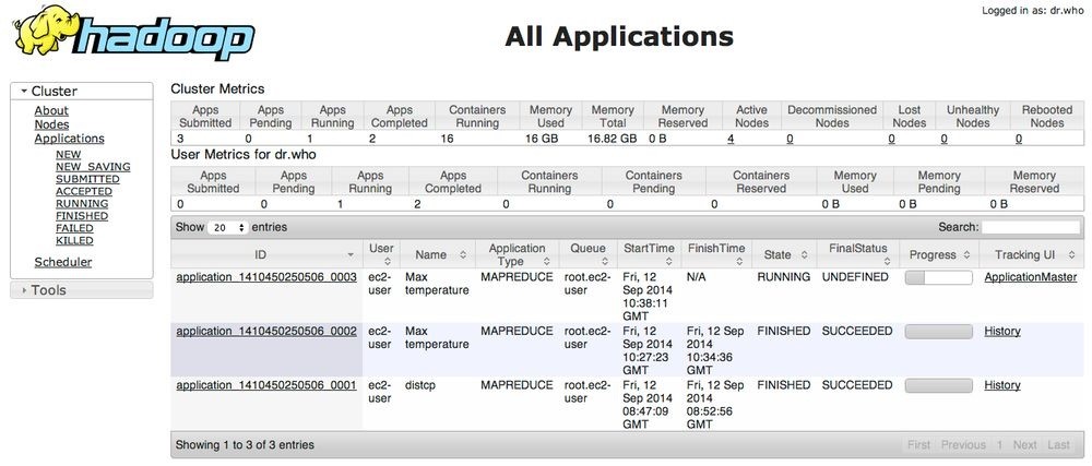
Figure 6-1. Screenshot of the resource manager page
The main table shows all the applications that have run or are currently running on the cluster. There is a search box that is useful for filtering the applications to find the ones you are interested in. The main view can show up to 100 entries per page, and the resource manager will keep up to 10,000 completed applications in memory at a time (set by yarn.resourcemanager.max-completed-applications), before they are only available from the job history page. Note also that the job history is persistent, so you can find jobs there from previous runs of the resource manager, too.
JOB HISTORY
Job history refers to the events and configuration for a completed MapReduce job. It is retained regardless of whether the job was successful, in an attempt to provide useful information for the user running a job.
Job history files are stored in HDFS by the MapReduce application master, in a directory set by the mapreduce.jobhistory.done-dir property. Job history files are kept for one week before being deleted by the system.
The history log includes job, task, and attempt events, all of which are stored in a file in JSON format. The history for a particular job may be viewed through the web UI for the job history server (which is linked to from the resource manager page) or via the command line using mapred job -history (which you point at the job history file).
The MapReduce job page
Clicking on the link for the “Tracking UI” takes us to the application master’s web UI (or to the history page if the application has completed). In the case of MapReduce, this takes us to the job page, illustrated in Figure 6-2.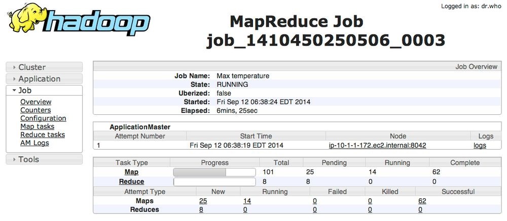
Figure 6-2. Screenshot of the job page
While the job is running, you can monitor its progress on this page. The table at the bottom shows the map progress and the reduce progress. “Total” shows the total number of map and reduce tasks for this job (a row for each). The other columns then show the state of these tasks: “Pending” (waiting to run), “Running,” or “Complete” (successfully run).
The lower part of the table shows the total number of failed and killed task attempts for the map or reduce tasks. Task attempts may be marked as killed if they are speculative execution duplicates, if the node they are running on dies, or if they are killed by a user. See Task Failure for background on task failure.
There also are a number of useful links in the navigation. For example, the
“Configuration” link is to the consolidated configuration file for the job, containing all the properties and their values that were in effect during the job run. If you are unsure of what a particular property was set to, you can click through to inspect the file.
Retrieving the Results
Once the job is finished, there are various ways to retrieve the results. Each reducer produces one output file, so there are 30 part files named part-r-00000 to part-r-00029 in the max-temp directory.
NOTE
As their names suggest, a good way to think of these “part” files is as parts of the max-temp “file.”
If the output is large (which it isn’t in this case), it is important to have multiple parts so that more than one reducer can work in parallel. Usually, if a file is in this partitioned form, it can still be used easily enough — as the input to another MapReduce job, for example. In some cases, you can exploit the structure of multiple partitions to do a mapside join, for example (see Map-Side Joins).
This job produces a very small amount of output, so it is convenient to copy it from HDFS to our development machine. The -getmerge option to the hadoop fs command is useful here, as it gets all the files in the directory specified in the source pattern and merges them into a single file on the local filesystem:
% hadoop fs -getmerge max-temp max-temp-local
% sort max-temp-local | tail
1991 607
1992 605
1993 567
1994 568
1995 567
1996 561
1997 565
1998 568
1999 568
2000 558
We sorted the output, as the reduce output partitions are unordered (owing to the hash partition function). Doing a bit of postprocessing of data from MapReduce is very common, as is feeding it into analysis tools such as R, a spreadsheet, or even a relational database.
Another way of retrieving the output if it is small is to use the -cat option to print the output files to the console:
% hadoop fs -cat max-temp/*
On closer inspection, we see that some of the results don’t look plausible. For instance, the maximum temperature for 1951 (not shown here) is 590°C! How do we find out what’s causing this? Is it corrupt input data or a bug in the program?
Debugging a Job
The time-honored way of debugging programs is via print statements, and this is certainly possible in Hadoop. However, there are complications to consider: with programs running on tens, hundreds, or thousands of nodes, how do we find and examine the output of the debug statements, which may be scattered across these nodes? For this particular case, where we are looking for (what we think is) an unusual case, we can use a debug statement to log to standard error, in conjunction with updating the task’s status message to prompt us to look in the error log. The web UI makes this easy, as we pass:[will see].
We also create a custom counter to count the total number of records with implausible temperatures in the whole dataset. This gives us valuable information about how to deal with the condition. If it turns out to be a common occurrence, we might need to learn more about the condition and how to extract the temperature in these cases, rather than simply dropping the records. In fact, when trying to debug a job, you should always ask yourself if you can use a counter to get the information you need to find out what’s happening. Even if you need to use logging or a status message, it may be useful to use a counter to gauge the extent of the problem. (There is more on counters in Counters.)
If the amount of log data you produce in the course of debugging is large, you have a couple of options. One is to write the information to the map’s output, rather than to standard error, for analysis and aggregation by the reduce task. This approach usually necessitates structural changes to your program, so start with the other technique first. The alternative is to write a program (in MapReduce, of course) to analyze the logs produced by your job.
We add our debugging to the mapper (version 3), as opposed to the reducer, as we want to find out what the source data causing the anomalous output looks like:
public class MaxTemperatureMapper
extends Mapper
enum Temperature {
OVER_100
}
private NcdcRecordParser parser = new NcdcRecordParser();
@Override
public void map(LongWritable key, Text value, Context context) throws IOException, InterruptedException {
parser.parse(value); if (parser.isValidTemperature()) { int airTemperature = parser.getAirTemperature(); if (airTemperature > 1000) {
System.err.println(“Temperature over 100 degrees for input: “ + value); context.setStatus(“Detected possibly corrupt record: see logs.”); context.getCounter(Temperature.OVER_100).increment(1);
} context.write(new Text(parser.getYear()), new IntWritable(airTemperature));
}
} }
If the temperature is over 100°C (represented by 1000, because temperatures are in tenths of a degree), we print a line to standard error with the suspect line, as well as updating the map’s status message using the setStatus() method on Context, directing us to look in the log. We also increment a counter, which in Java is represented by a field of an enum type. In this program, we have defined a single field, OVER_100, as a way to count the number of records with a temperature of over 100°C.
With this modification, we recompile the code, re-create the JAR file, then rerun the job and, while it’s running, go to the tasks page.
The tasks and task attempts pages
The job page has a number of links for viewing the tasks in a job in more detail. For example, clicking on the “Map” link brings us to a page that lists information for all of the map tasks. The screenshot in Figure 6-3 shows this page for the job run with our debugging statements in the “Status” column for the task.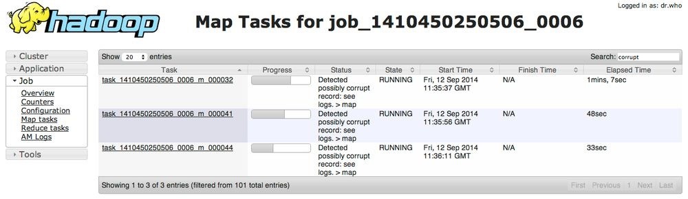
Figure 6-3. Screenshot of the tasks page
Clicking on the task link takes us to the task attempts page, which shows each task attempt for the task. Each task attempt page has links to the logfiles and counters. If we follow one of the links to the logfiles for the successful task attempt, we can find the suspect input record that we logged (the line is wrapped and truncated to fit on the page):
Temperature over 100 degrees for input:
0335999999433181957042302005+37950+139117SAO +0004RJSN V02011359003150070356999 999433201957010100005+35317+139650SAO +000899999V02002359002650076249N0040005…
This record seems to be in a different format from the others. For one thing, there are spaces in the line, which are not described in the specification.
When the job has finished, we can look at the value of the counter we defined to see how many records over 100°C there are in the whole dataset. Counters are accessible via the web UI or the command line:
% mapred job -counter job_1410450250506_0006 \
‘v3.MaxTemperatureMapper$Temperature’ OVER_100 3
The -counter option takes the job ID, counter group name (which is the fully qualified classname here), and counter name (the enum name). There are only three malformed records in the entire dataset of over a billion records. Throwing out bad records is standard for many big data problems, although we need to be careful in this case because we are looking for an extreme value — the maximum temperature rather than an aggregate measure. Still, throwing away three records is probably not going to change the result.
Handling malformed data
Capturing input data that causes a problem is valuable, as we can use it in a test to check that the mapper does the right thing. In this MRUnit test, we check that the counter is updated for the malformed input:
@Test
public void parsesMalformedTemperature() throws IOException,
InterruptedException {
Text value = new Text(“0335999999433181957042302005+37950+139117SAO +0004” +
// Year ^^^^
“RJSN V02011359003150070356999999433201957010100005+353”);
// Temperature ^^^^^ Counters counters = new Counters();
new MapDriver
.withMapper(new MaxTemperatureMapper())
.withInput(new LongWritable(0), value)
.withCounters(counters)
.runTest();
Counter c = counters.findCounter(MaxTemperatureMapper.Temperature.MALFORMED); assertThat(c.getValue(), is(1L)); }
The record that was causing the problem is of a different format than the other lines we’ve seen. Example 6-12 shows a modified program (version 4) using a parser that ignores each line with a temperature field that does not have a leading sign (plus or minus). We’ve also introduced a counter to measure the number of records that we are ignoring for this reason.
Example 6-12. Mapper for the maximum temperature example
public class MaxTemperatureMapper extends Mapper
enum Temperature {
MALFORMED
}
private NcdcRecordParser parser = new NcdcRecordParser();
@Override
public void map(LongWritable key, Text value, Context context) throws IOException, InterruptedException {
parser.parse(value); if (parser.isValidTemperature()) { int airTemperature = parser.getAirTemperature(); context.write(new Text(parser.getYear()), new IntWritable(airTemperature));
} else if (parser.isMalformedTemperature()) {
System.err.println(“Ignoring possibly corrupt input: “ + value); context.getCounter(Temperature.MALFORMED).increment(1); }
} }
Hadoop Logs
Hadoop produces logs in various places, and for various audiences. These are summarized in Table 6-2.
Table 6-2. Types of Hadoop logs
| Logs Primary audience | Description | Further information |
|---|---|---|
| System Administrators daemon logs |
Each Hadoop daemon produces a logfile (using log4j) and another file that combines standard out and error. Written in the directory defined by the HADOOP_LOG_DIR environment variable. | System logfiles and Logging |
| HDFS audit Administrators logs | A log of all HDFS requests, turned off by default. Written to the namenode’s log, although this is configurable. | Audit Logging |
MapReduce Users A log of the events (such as task completion) that occur in the course of Job History job history running a job. Saved centrally in HDFS.
logs
| MapReduce Users task logs |
Each task child process produces a logfile using log4j (called syslog), a file for data sent to standard out (stdout), and a file for standard error (stderr). Written in the userlogs subdirectory of the directory defined by the YARN_LOG_DIR environment variable. | This section |
|---|---|---|
YARN has a service for log aggregation that takes the task logs for completed applications and moves them to HDFS, where they are stored in a container file for archival purposes.
If this service is enabled (by setting yarn.log-aggregation-enable to true on the cluster), then task logs can be viewed by clicking on the logs link in the task attempt web UI, or by using the mapred job -logs command.
By default, log aggregation is not enabled. In this case, task logs can be retrieved by visiting the node manager’s web UI at http://__node-manager-host:8042/logs/userlogs.
It is straightforward to write to these logfiles. Anything written to standard output or standard error is directed to the relevant logfile. (Of course, in Streaming, standard output is used for the map or reduce output, so it will not show up in the standard output log.)
In Java, you can write to the task’s syslog file if you wish by using the Apache Commons Logging API (or indeed any logging API that can write to log4j). This is shown in Example 6-13.
Example 6-13. An identity mapper that writes to standard output and also uses the Apache Commons Logging API
import org.apache.commons.logging.Log; import org.apache.commons.logging.LogFactory; import org.apache.hadoop.mapreduce.Mapper;
public class LoggingIdentityMapper
private static final Log LOG = LogFactory.getLog(LoggingIdentityMapper.class); @Override
@SuppressWarnings(“unchecked”)
public void map(KEYIN key, VALUEIN value, Context context) throws IOException, InterruptedException {
// Log to stdout file
System.out.println(“Map key: “ + key);
// Log to syslog file LOG.info(“Map key: “ + key); if (LOG.isDebugEnabled()) {
LOG.debug(“Map value: “ + value);
}
context.write((KEYOUT) key, (VALUEOUT) value);
} }
The default log level is INFO, so DEBUG-level messages do not appear in the syslog task logfile. However, sometimes you want to see these messages. To enable this, set mapreduce.map.log.level or mapreduce.reduce.log.level, as appropriate. For example, in this case, we could set it for the mapper to see the map values in the log as follows:
% hadoop jar hadoop-examples.jar LoggingDriver -conf conf/hadoop-cluster.xml \
-D mapreduce.map.log.level=DEBUG input/ncdc/sample.txt logging-out
There are some controls for managing the retention and size of task logs. By default, logs are deleted after a minimum of three hours (you can set this using the yarn.nodemanager.log.retain-seconds property, although this is ignored if log aggregation is enabled). You can also set a cap on the maximum size of each logfile using the mapreduce.task.userlog.limit.kb property, which is 0 by default, meaning there is no cap.
TIP
Sometimes you may need to debug a problem that you suspect is occurring in the JVM running a Hadoop command, rather than on the cluster. You can send DEBUG-level logs to the console by using an invocation like this: % HADOOP_ROOT_LOGGER=DEBUG,console hadoop fs -text /foo/bar
Remote Debugging
When a task fails and there is not enough information logged to diagnose the error, you may want to resort to running a debugger for that task. This is hard to arrange when running the job on a cluster, as you don’t know which node is going to process which part of the input, so you can’t set up your debugger ahead of the failure. However, there are a few other options available:
Reproduce the failure locally
Often the failing task fails consistently on a particular input. You can try to reproduce the problem locally by downloading the file that the task is failing on and running the job locally, possibly using a debugger such as Java’s VisualVM.
Use JVM debugging options
A common cause of failure is a Java out of memory error in the task JVM. You can set mapred.child.java.opts to include -XX:-HeapDumpOnOutOfMemoryError XX:HeapDumpPath=/path/to/dumps. This setting produces a heap dump that can be examined afterward with tools such as jhat or the Eclipse Memory Analyzer. Note that the JVM options should be added to the existing memory settings specified by mapred.child.java.opts. These are explained in more detail in Memory settings in YARN and MapReduce.
Use task profiling
Java profilers give a lot of insight into the JVM, and Hadoop provides a mechanism to profile a subset of the tasks in a job. See Profiling Tasks.
In some cases, it’s useful to keep the intermediate files for a failed task attempt for later inspection, particularly if supplementary dump or profile files are created in the task’s working directory. You can set mapreduce.task.files.preserve.failedtasks to true to keep a failed task’s files.
You can keep the intermediate files for successful tasks, too, which may be handy if you want to examine a task that isn’t failing. In this case, set the property
mapreduce.task.files.preserve.filepattern to a regular expression that matches the IDs of the tasks whose files you want to keep.
Another useful property for debugging is yarn.nodemanager.delete.debug-delay-sec, which is the number of seconds to wait to delete localized task attempt files, such as the script used to launch the task container JVM. If this is set on the cluster to a reasonably large value (e.g., 600 for 10 minutes), then you have enough time to look at the files before they are deleted.
To examine task attempt files, log into the node that the task failed on and look for the directory for that task attempt. It will be under one of the local MapReduce directories, as set by the mapreduce.cluster.local.dir property (covered in more detail in Important Hadoop Daemon Properties). If this property is a comma-separated list of directories (to spread load across the physical disks on a machine), you may need to look in all of the directories before you find the directory for that particular task attempt. The task attempt directory is in the following location:
mapreduce.cluster.local.dir/usercache/user/appcache/application-ID/output /task-attempt-ID
Tuning a Job
After a job is working, the question many developers ask is, “Can I make it run faster?”
There are a few Hadoop-specific “usual suspects” that are worth checking to see whether they are responsible for a performance problem. You should run through the checklist in Table 6-3 before you start trying to profile or optimize at the task level. Table 6-3. Tuning checklist
| Area | Best practice | Further information |
|---|---|---|
| Number of mappers | How long are your mappers running for? If they are only running for a few seconds on average, you should see whether there’s a way to have fewer mappers and make them all run longer — a minute or so, as a rule of thumb. The extent to which this is possible depends on the input format you are using. | Small files and CombineFileInputFormat |
| Number of reducers | Check that you are using more than a single reducer. Reduce tasks should run for five minutes or so and produce at least a block’s worth of data, as a rule of thumb. | Choosing the Number of Reducers |
| Combiners | Check whether your job can take advantage of a combiner to reduce the amount of data passing through the shuffle. | Combiner Functions |
| Intermediate compression | Job execution time can almost always benefit from enabling map output compression. | Compressing map output |
| Custom serialization |
If you are using your own custom Writable objects or custom comparators, make sure you have implemented RawComparator. | Implementing a RawComparator for speed |
| Shuffle tweaks | The MapReduce shuffle exposes around a dozen tuning parameters for memory management, which may help you wring out the last bit of performance. | Configuration Tuning |
Profiling Tasks
Like debugging, profiling a job running on a distributed system such as MapReduce presents some challenges. Hadoop allows you to profile a fraction of the tasks in a job and, as each task completes, pulls down the profile information to your machine for later analysis with standard profiling tools.
Of course, it’s possible, and somewhat easier, to profile a job running in the local job runner. And provided you can run with enough input data to exercise the map and reduce tasks, this can be a valuable way of improving the performance of your mappers and reducers. There are a couple of caveats, however. The local job runner is a very different environment from a cluster, and the data flow patterns are very different. Optimizing the CPU performance of your code may be pointless if your MapReduce job is I/O-bound (as many jobs are). To be sure that any tuning is effective, you should compare the new execution time with the old one running on a real cluster. Even this is easier said than done, since job execution times can vary due to resource contention with other jobs and the decisions the scheduler makes regarding task placement. To get a good idea of job execution time under these circumstances, perform a series of runs (with and without the change) and check whether any improvement is statistically significant.
It’s unfortunately true that some problems (such as excessive memory use) can be reproduced only on the cluster, and in these cases the ability to profile in situ is indispensable.
The HPROF profiler
There are a number of configuration properties to control profiling, which are also exposed via convenience methods on JobConf. Enabling profiling is as simple as setting the property mapreduce.task.profile to true:
% hadoop jar hadoop-examples.jar v4.MaxTemperatureDriver \
-conf conf/hadoop-cluster.xml \
-D mapreduce.task.profile=true \ input/ncdc/all max-temp
This runs the job as normal, but adds an -agentlib parameter to the Java command used to launch the task containers on the node managers. You can control the precise parameter that is added by setting the mapreduce.task.profile.params property. The default uses HPROF, a profiling tool that comes with the JDK that, although basic, can give valuable information about a program’s CPU and heap usage.
It doesn’t usually make sense to profile all tasks in the job, so by default only those with IDs 0, 1, and 2 are profiled (for both maps and reduces). You can change this by setting mapreduce.task.profile.maps and mapreduce.task.profile.reduces to specify the range of task IDs to profile.
The profile output for each task is saved with the task logs in the userlogs subdirectory of the node manager’s local log directory (alongside the syslog, stdout, and stderr files), and can be retrieved in the way described in Hadoop Logs, according to whether log aggregation is enabled or not.
MapReduce Workflows
So far in this chapter, you have seen the mechanics of writing a program using MapReduce. We haven’t yet considered how to turn a data processing problem into the MapReduce model.
The data processing you have seen so far in this book is to solve a fairly simple problem: finding the maximum recorded temperature for given years. When the processing gets more complex, this complexity is generally manifested by having more MapReduce jobs, rather than having more complex map and reduce functions. In other words, as a rule of thumb, think about adding more jobs, rather than adding complexity to jobs.
For more complex problems, it is worth considering a higher-level language than MapReduce, such as Pig, Hive, Cascading, Crunch, or Spark. One immediate benefit is that it frees you from having to do the translation into MapReduce jobs, allowing you to concentrate on the analysis you are performing.
Finally, the book Data-Intensive Text Processing with MapReduce by Jimmy Lin and Chris Dyer (Morgan & Claypool Publishers, 2010) is a great resource for learning more about MapReduce algorithm design and is highly recommended.
Decomposing a Problem into MapReduce Jobs
Let’s look at an example of a more complex problem that we want to translate into a MapReduce workflow.
Imagine that we want to find the mean maximum recorded temperature for every day of the year and every weather station. In concrete terms, to calculate the mean maximum daily temperature recorded by station 029070-99999, say, on January 1, we take the mean of the maximum daily temperatures for this station for January 1, 1901; January 1, 1902; and so on, up to January 1, 2000.
How can we compute this using MapReduce? The computation decomposes most naturally into two stages:
1. Compute the maximum daily temperature for every station-date pair.
The MapReduce program in this case is a variant of the maximum temperature program, except that the keys in this case are a composite station-date pair, rather than just the year.
2. Compute the mean of the maximum daily temperatures for every station-day-month key.
The mapper takes the output from the previous job (station-date, maximum temperature) records and projects it into (station-day-month, maximum temperature) records by dropping the year component. The reduce function then takes the mean of the maximum temperatures for each station-day-month key.
The output from the first stage looks like this for the station we are interested in (the mean_max_daily_temp.sh script in the examples provides an implementation in Hadoop Streaming):
029070-99999 19010101 0
029070-99999 19020101 -94…
The first two fields form the key, and the final column is the maximum temperature from all the readings for the given station and date. The second stage averages these daily maxima over years to yield:
029070-99999 0101 -68 which is interpreted as saying the mean maximum daily temperature on January 1 for station 029070-99999 over the century is −6.8°C.
It’s possible to do this computation in one MapReduce stage, but it takes more work on the part of the programmer.50]
The arguments for having more (but simpler) MapReduce stages are that doing so leads to more composable and more maintainable mappers and reducers. Some of the case studies referred to in Part V cover real-world problems that were solved using MapReduce, and in each case, the data processing task is implemented using two or more MapReduce jobs. The details in that chapter are invaluable for getting a better idea of how to decompose a processing problem into a MapReduce workflow.
It’s possible to make map and reduce functions even more composable than we have done. A mapper commonly performs input format parsing, projection (selecting the relevant fields), and filtering (removing records that are not of interest). In the mappers you have seen so far, we have implemented all of these functions in a single mapper. However, there is a case for splitting these into distinct mappers and chaining them into a single mapper using the ChainMapper library class that comes with Hadoop. Combined with a
ChainReducer, you can run a chain of mappers, followed by a reducer and another chain of mappers, in a single MapReduce job.
JobControl
When there is more than one job in a MapReduce workflow, the question arises: how do you manage the jobs so they are executed in order? There are several approaches, and the main consideration is whether you have a linear chain of jobs or a more complex directed acyclic graph (DAG) of jobs.
For a linear chain, the simplest approach is to run each job one after another, waiting until a job completes successfully before running the next:
JobClient.runJob(conf1);
JobClient.runJob(conf2);
If a job fails, the runJob() method will throw an IOException, so later jobs in the pipeline don’t get executed. Depending on your application, you might want to catch the exception and clean up any intermediate data that was produced by any previous jobs.
The approach is similar with the new MapReduce API, except you need to examine the Boolean return value of the waitForCompletion() method on Job: true means the job succeeded, and false means it failed.
For anything more complex than a linear chain, there are libraries that can help orchestrate your workflow (although they are also suited to linear chains, or even one-off jobs). The simplest is in the org.apache.hadoop.mapreduce.jobcontrol package: the JobControl class. (There is an equivalent class in the org.apache.hadoop.mapred.jobcontrol package, too.) An instance of JobControl represents a graph of jobs to be run. You add
the job configurations, then tell the JobControl instance the dependencies between jobs. You run the JobControl in a thread, and it runs the jobs in dependency order. You can poll for progress, and when the jobs have finished, you can query for all the jobs’ statuses and the associated errors for any failures. If a job fails, JobControl won’t run its dependencies.
Apache Oozie
Apache Oozie is a system for running workflows of dependent jobs. It is composed of two main parts: a workflow engine that stores and runs workflows composed of different types of Hadoop jobs (MapReduce, Pig, Hive, and so on), and a coordinator engine that runs workflow jobs based on predefined schedules and data availability. Oozie has been designed to scale, and it can manage the timely execution of thousands of workflows in a Hadoop cluster, each composed of possibly dozens of constituent jobs.
Oozie makes rerunning failed workflows more tractable, since no time is wasted running successful parts of a workflow. Anyone who has managed a complex batch system knows how difficult it can be to catch up from jobs missed due to downtime or failure, and will appreciate this feature. (Furthermore, coordinator applications representing a single data pipeline may be packaged into a bundle and run together as a unit.)
Unlike JobControl, which runs on the client machine submitting the jobs, Oozie runs as a service in the cluster, and clients submit workflow definitions for immediate or later execution. In Oozie parlance, a workflow is a DAG of action nodes and control-flow nodes.
An action node performs a workflow task, such as moving files in HDFS; running a MapReduce, Streaming, Pig, or Hive job; performing a Sqoop import; or running an arbitrary shell script or Java program. A control-flow node governs the workflow execution between actions by allowing such constructs as conditional logic (so different execution branches may be followed depending on the result of an earlier action node) or parallel execution. When the workflow completes, Oozie can make an HTTP callback to the client to inform it of the workflow status. It is also possible to receive callbacks every time the workflow enters or exits an action node.
Defining an Oozie workflow
Workflow definitions are written in XML using the Hadoop Process Definition Language, the specification for which can be found on the Oozie website. Example 6-14 shows a simple Oozie workflow definition for running a single MapReduce job.
Example 6-14. Oozie workflow definition to run the maximum temperature MapReduce job
<workflow-app xmlns=”uri:oozie:workflow:0.1” name=”max-temp-workflow”>
<start to=”max-temp-mr”/>
<action name=”max-temp-mr”>
<delete path=”${nameNode}/user/${wf:user()}/output”/>
<ok to=”end”/>
<error to=”fail”/>
<kill name=”fail”>
<end name=”end”/>
This workflow has three control-flow nodes and one action node: a start control node, a map-reduce action node, a kill control node, and an end control node. The nodes and allowed transitions between them are shown in Figure 6-4.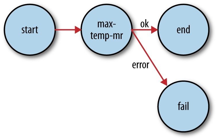
Figure 6-4. Transition diagram of an Oozie workflow
All workflows must have one start and one end node. When the workflow job starts, it transitions to the node specified by the start node (the max-temp-mr action in this example). A workflow job succeeds when it transitions to the end node. However, if the workflow job transitions to a kill node, it is considered to have failed and reports the appropriate error message specified by the message element in the workflow definition.
The bulk of this workflow definition file specifies the map-reduce action. The first two elements, job-tracker and name-node, are used to specify the YARN resource manager (or jobtracker in Hadoop 1) to submit the job to and the namenode (actually a Hadoop filesystem URI) for input and output data. Both are parameterized so that the workflow definition is not tied to a particular cluster (which makes it easy to test). The parameters are specified as workflow job properties at submission time, as we shall see later.
The optional prepare element runs before the MapReduce job and is used for directory deletion (and creation, too, if needed, although that is not shown here). By ensuring that the output directory is in a consistent state before running a job, Oozie can safely rerun the action if the job fails.
The MapReduce job to run is specified in the configuration element using nested elements for specifying the Hadoop configuration name-value pairs. You can view the MapReduce configuration section as a declarative replacement for the driver classes that we have used elsewhere in this book for running MapReduce programs (such as Example 2-5).
We have taken advantage of JSP Expression Language (EL) syntax in several places in the workflow definition. Oozie provides a set of functions for interacting with the workflow.
For example, ${wf:user()} returns the name of the user who started the current workflow job, and we use it to specify the correct filesystem path. The Oozie specification lists all the EL functions that Oozie supports.
Packaging and deploying an Oozie workflow application
A workflow application is made up of the workflow definition plus all the associated resources (such as MapReduce JAR files, Pig scripts, and so on) needed to run it. Applications must adhere to a simple directory structure, and are deployed to HDFS so that they can be accessed by Oozie. For this workflow application, we’ll put all of the files in a base directory called max-temp-workflow, as shown diagrammatically here:
max-temp-workflow/
├── lib/
│ └── hadoop-examples.jar └── workflow.xml
The workflow definition file workflow.xml must appear in the top level of this directory.
JAR files containing the application’s MapReduce classes are placed in the lib directory.
Workflow applications that conform to this layout can be built with any suitable build tool, such as Ant or Maven; you can find an example in the code that accompanies this book. Once an application has been built, it should be copied to HDFS using regular Hadoop tools. Here is the appropriate command for this application:
% hadoop fs -put hadoop-examples/target/max-temp-workflow max-temp-workflow
Running an Oozie workflow job
Next, let’s see how to run a workflow job for the application we just uploaded. For this we use the oozie command-line tool, a client program for communicating with an Oozie server. For convenience, we export the OOZIEURL environment variable to tell the oozie command which Oozie server to use (here we’re using one running locally):
% export OOZIE_URL=”http://localhost:11000/oozie“
There are lots of subcommands for the _oozie tool (type oozie help to get a list), but we’re going to call the job subcommand with the -run option to run the workflow job:
% oozie job -config ch06-mr-dev/src/main/resources/max-temp-workflow.properties \
-run job: 0000001-140911033236814-oozie-oozi-W
The -config option specifies a local Java properties file containing definitions for the parameters in the workflow XML file (in this case, nameNode and resourceManager), as well as oozie.wf.application.path, which tells Oozie the location of the workflow application in HDFS. Here are the contents of the properties file:
nameNode=hdfs://localhost:8020 resourceManager=localhost:8032 oozie.wf.application.path=${nameNode}/user/${user.name}/max-temp-workflow
To get information about the status of the workflow job, we use the -info option, specifying the job ID that was printed by the run command earlier (type oozie job to get a list of all jobs):
% oozie job -info 0000001-140911033236814-oozie-oozi-W
The output shows the status: RUNNING, KILLED, or SUCCEEDED. You can also find all this information via Oozie’s web UI (http://localhost:11000/oozie).
When the job has succeeded, we can inspect the results in the usual way:
% hadoop fs -cat output/part-*
1949 111
1950 22
This example only scratched the surface of writing Oozie workflows. The documentation on Oozie’s website has information about creating more complex workflows, as well as writing and running coordinator jobs.
[49] In Hadoop 1, mapred.job.tracker determines the means of execution: local for the local job runner, or a colonseparated host and port pair for a jobtracker address.
[50] It’s an interesting exercise to do this. Hint: use Secondary Sort.
Chapter 7. How MapReduce Works
In this chapter, we look at how MapReduce in Hadoop works in detail. This knowledge provides a good foundation for writing more advanced MapReduce programs, which we will cover in the following two chapters.
Anatomy of a MapReduce Job Run
You can run a MapReduce job with a single method call: submit() on a Job object (you can also call waitForCompletion(), which submits the job if it hasn’t been submitted already, then waits for it to finish).51] This method call conceals a great deal of processing behind the scenes. This section uncovers the steps Hadoop takes to run a job.
The whole process is illustrated in Figure 7-1. At the highest level, there are five independent entities:52]
The client, which submits the MapReduce job.
The YARN resource manager, which coordinates the allocation of compute resources on the cluster.
The YARN node managers, which launch and monitor the compute containers on machines in the cluster.
The MapReduce application master, which coordinates the tasks running the MapReduce job. The application master and the MapReduce tasks run in containers that are scheduled by the resource manager and managed by the node managers. The distributed filesystem (normally HDFS, covered in Chapter 3), which is used for sharing job files between the other entities.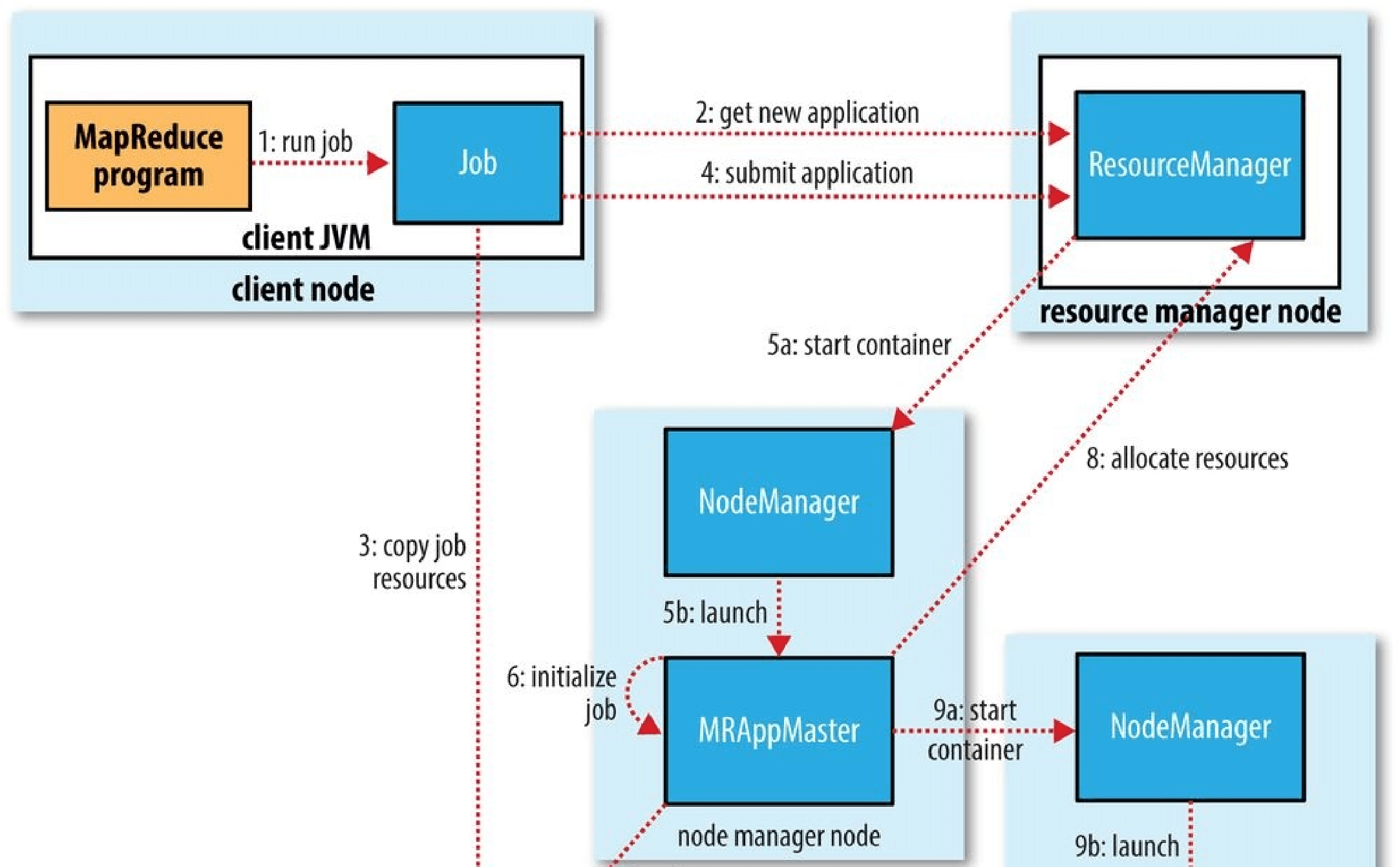
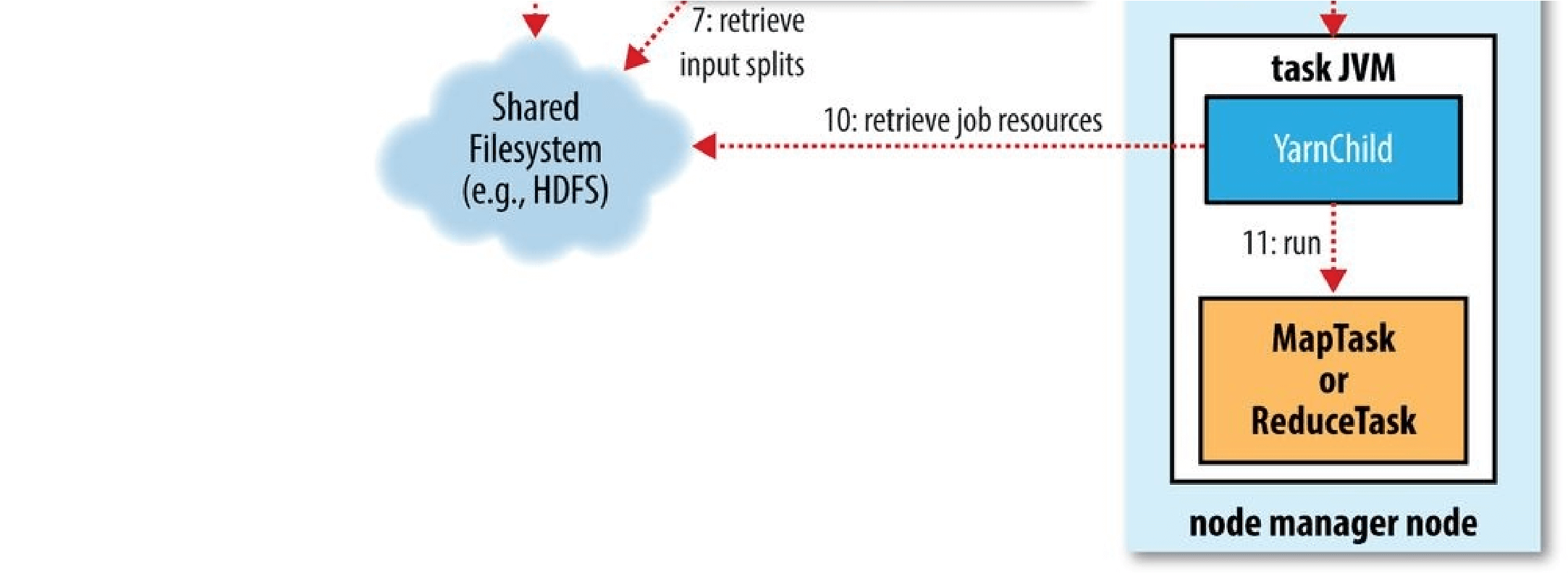
Figure 7-1. How Hadoop runs a MapReduce job
Job Submission
The submit() method on Job creates an internal JobSubmitter instance and calls submitJobInternal() on it (step 1 in Figure 7-1). Having submitted the job,
waitForCompletion() polls the job’s progress once per second and reports the progress to the console if it has changed since the last report. When the job completes successfully, the job counters are displayed. Otherwise, the error that caused the job to fail is logged to the console.
The job submission process implemented by JobSubmitter does the following:
Asks the resource manager for a new application ID, used for the MapReduce job ID (step 2).
Checks the output specification of the job. For example, if the output directory has not been specified or it already exists, the job is not submitted and an error is thrown to the MapReduce program. Computes the input splits for the job. If the splits cannot be computed (because the input paths don’t exist, for example), the job is not submitted and an error is thrown to the MapReduce program. Copies the resources needed to run the job, including the job JAR file, the configuration file, and the computed input splits, to the shared filesystem in a directory named after the job ID (step 3). The job JAR is copied with a high replication factor
(controlled by the mapreduce.client.submit.file.replication property, which defaults to 10) so that there are lots of copies across the cluster for the node managers to access when they run tasks for the job. Submits the job by calling submitApplication() on the resource manager (step 4).
Job Initialization
When the resource manager receives a call to its submitApplication() method, it hands off the request to the YARN scheduler. The scheduler allocates a container, and the resource manager then launches the application master’s process there, under the node manager’s management (steps 5a and 5b).
The application master for MapReduce jobs is a Java application whose main class is
MRAppMaster. It initializes the job by creating a number of bookkeeping objects to keep track of the job’s progress, as it will receive progress and completion reports from the tasks (step 6). Next, it retrieves the input splits computed in the client from the shared filesystem (step 7). It then creates a map task object for each split, as well as a number of reduce task objects determined by the mapreduce.job.reduces property (set by the setNumReduceTasks() method on Job). Tasks are given IDs at this point.
The application master must decide how to run the tasks that make up the MapReduce job. If the job is small, the application master may choose to run the tasks in the same JVM as itself. This happens when it judges that the overhead of allocating and running tasks in new containers outweighs the gain to be had in running them in parallel, compared to running them sequentially on one node. Such a job is said to be uberized, or run as an uber task.
What qualifies as a small job? By default, a small job is one that has less than 10 mappers, only one reducer, and an input size that is less than the size of one HDFS block. (Note that these values may be changed for a job by setting mapreduce.job.ubertask.maxmaps,
mapreduce.job.ubertask.maxreduces, and mapreduce.job.ubertask.maxbytes.) Uber tasks must be enabled explicitly (for an individual job, or across the cluster) by setting mapreduce.job.ubertask.enable to true.
Finally, before any tasks can be run, the application master calls the setupJob() method on the OutputCommitter. For FileOutputCommitter, which is the default, it will create the final output directory for the job and the temporary working space for the task output. The commit protocol is described in more detail in Output Committers.
Task Assignment
If the job does not qualify for running as an uber task, then the application master requests containers for all the map and reduce tasks in the job from the resource manager (step 8). Requests for map tasks are made first and with a higher priority than those for reduce tasks, since all the map tasks must complete before the sort phase of the reduce can start (see Shuffle and Sort). Requests for reduce tasks are not made until 5% of map tasks have completed (see Reduce slow start).
Reduce tasks can run anywhere in the cluster, but requests for map tasks have data locality constraints that the scheduler tries to honor (see Resource Requests). In the optimal case, the task is data local — that is, running on the same node that the split resides on. Alternatively, the task may be rack local: on the same rack, but not the same node, as the split. Some tasks are neither data local nor rack local and retrieve their data from a different rack than the one they are running on. For a particular job run, you can determine the number of tasks that ran at each locality level by looking at the job’s counters (see Table 9-6).
Requests also specify memory requirements and CPUs for tasks. By default, each map and reduce task is allocated 1,024 MB of memory and one virtual core. The values are configurable on a per-job basis (subject to minimum and maximum values described in Memory settings in YARN and MapReduce) via the following properties: mapreduce.map.memory.mb, mapreduce.reduce.memory.mb, mapreduce.map.cpu.vcores and mapreduce.reduce.cpu.vcores.
Task Execution
Once a task has been assigned resources for a container on a particular node by the resource manager’s scheduler, the application master starts the container by contacting the node manager (steps 9a and 9b). The task is executed by a Java application whose main class is YarnChild. Before it can run the task, it localizes the resources that the task needs, including the job configuration and JAR file, and any files from the distributed cache (step 10; see Distributed Cache). Finally, it runs the map or reduce task (step 11).
The YarnChild runs in a dedicated JVM, so that any bugs in the user-defined map and reduce functions (or even in YarnChild) don’t affect the node manager — by causing it to crash or hang, for example.
Each task can perform setup and commit actions, which are run in the same JVM as the task itself and are determined by the OutputCommitter for the job (see Output Committers). For file-based jobs, the commit action moves the task output from a temporary location to its final location. The commit protocol ensures that when speculative execution is enabled (see Speculative Execution), only one of the duplicate tasks is committed and the other is aborted.
Streaming
Streaming runs special map and reduce tasks for the purpose of launching the usersupplied executable and communicating with it (Figure 7-2).
The Streaming task communicates with the process (which may be written in any language) using standard input and output streams. During execution of the task, the Java process passes input key-value pairs to the external process, which runs it through the user-defined map or reduce function and passes the output key-value pairs back to the Java process. From the node manager’s point of view, it is as if the child process ran the map or reduce code itself.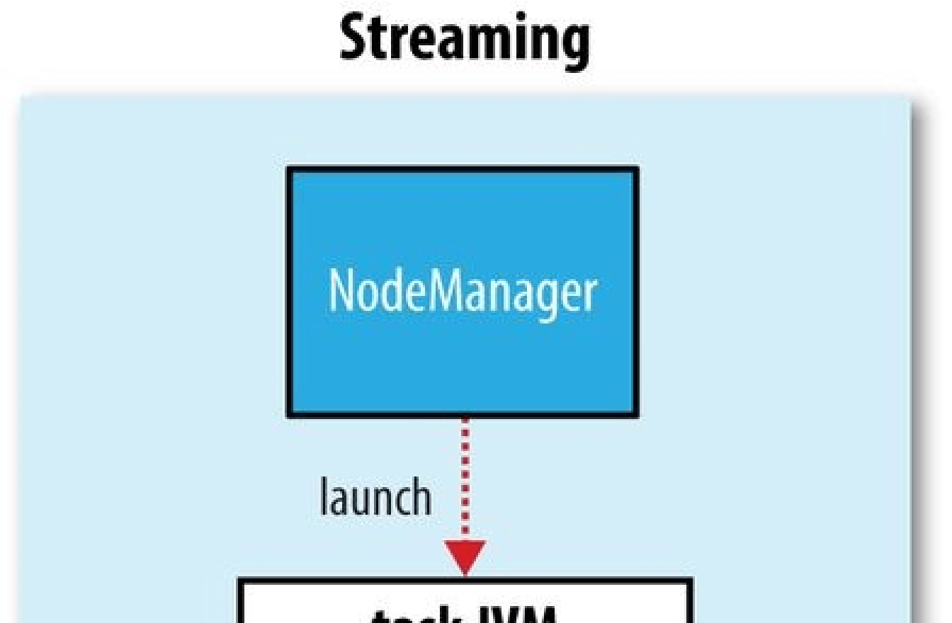
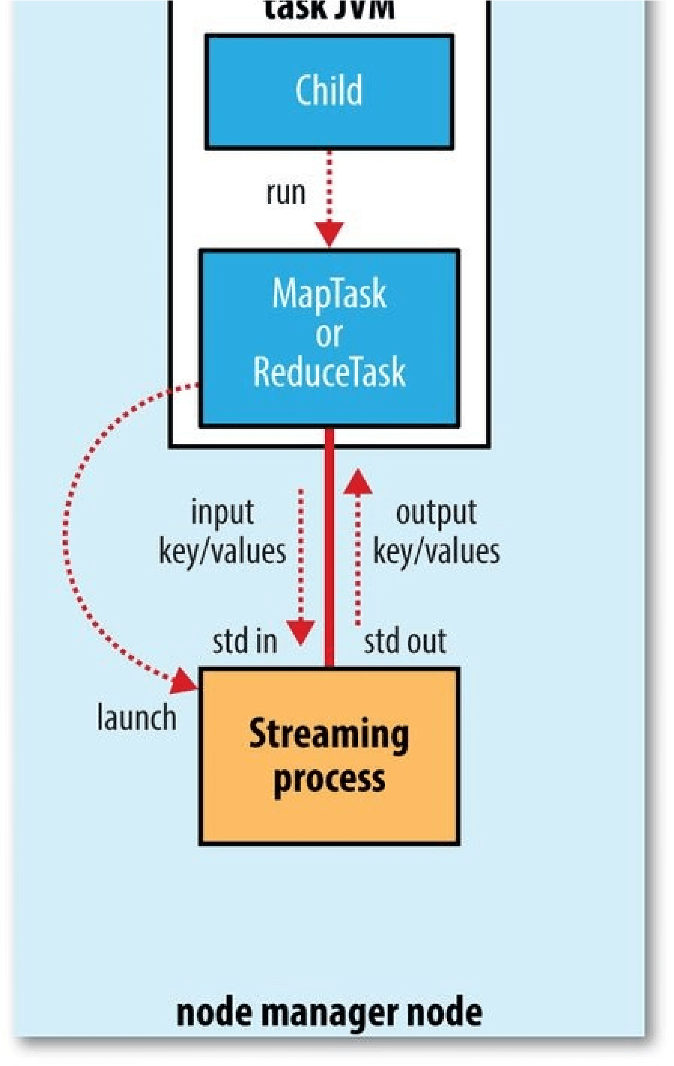
Figure 7-2. The relationship of the Streaming executable to the node manager and the task container
Progress and Status Updates
MapReduce jobs are long-running batch jobs, taking anything from tens of seconds to hours to run. Because this can be a significant length of time, it’s important for the user to get feedback on how the job is progressing. A job and each of its tasks have a status, which includes such things as the state of the job or task (e.g., running, successfully completed, failed), the progress of maps and reduces, the values of the job’s counters, and a status message or description (which may be set by user code). These statuses change over the course of the job, so how do they get communicated back to the client?
When a task is running, it keeps track of its progress (i.e., the proportion of the task completed). For map tasks, this is the proportion of the input that has been processed. For reduce tasks, it’s a little more complex, but the system can still estimate the proportion of the reduce input processed. It does this by dividing the total progress into three parts, corresponding to the three phases of the shuffle (see Shuffle and Sort). For example, if the task has run the reducer on half its input, the task’s progress is 5/6, since it has completed the copy and sort phases (1/3 each) and is halfway through the reduce phase (1/6).
WHAT CONSTITUTES PROGRESS IN MAPREDUCE?
Progress is not always measurable, but nevertheless, it tells Hadoop that a task is doing something. For example, a task writing output records is making progress, even when it cannot be expressed as a percentage of the total number that will be written (because the latter figure may not be known, even by the task producing the output).
Progress reporting is important, as Hadoop will not fail a task that’s making progress. All of the following operations constitute progress:
Reading an input record (in a mapper or reducer)
Writing an output record (in a mapper or reducer)
Setting the status description (via Reporter’s or TaskAttemptContext’s setStatus() method)
Incrementing a counter (using Reporter’s incrCounter() method or Counter’s increment() method) Calling Reporter’s or TaskAttemptContext’s progress() method
Tasks also have a set of counters that count various events as the task runs (we saw an example in A test run), which are either built into the framework, such as the number of map output records written, or defined by users.
As the map or reduce task runs, the child process communicates with its parent application master through the umbilical interface. The task reports its progress and status (including counters) back to its application master, which has an aggregate view of the job, every three seconds over the umbilical interface.
The resource manager web UI displays all the running applications with links to the web UIs of their respective application masters, each of which displays further details on the MapReduce job, including its progress.
During the course of the job, the client receives the latest status by polling the application master every second (the interval is set via mapreduce.client.progressmonitor.pollinterval). Clients can also use Job’s getStatus() method to obtain a JobStatus instance, which contains all of the status information for the job.
The process is illustrated in Figure 7-3.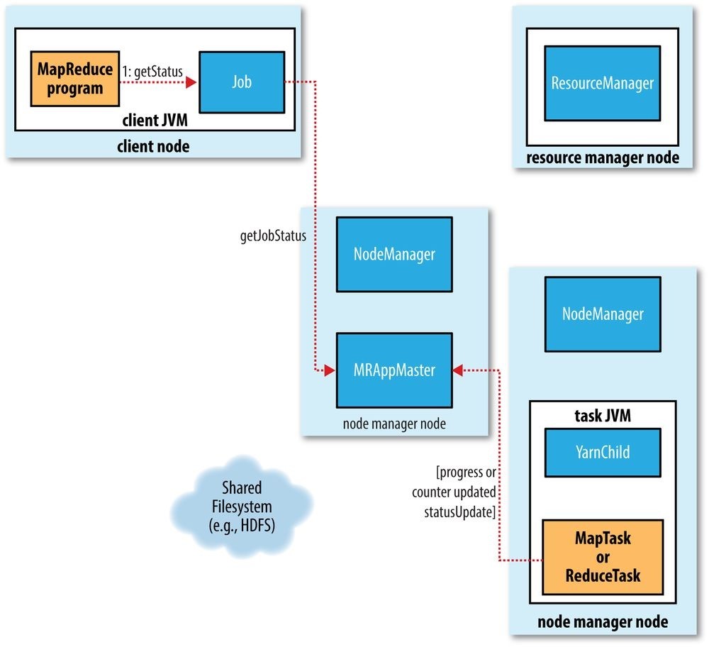
Figure 7-3. How status updates are propagated through the MapReduce system
Job Completion
When the application master receives a notification that the last task for a job is complete, it changes the status for the job to “successful.” Then, when the Job polls for status, it learns that the job has completed successfully, so it prints a message to tell the user and then returns from the waitForCompletion() method. Job statistics and counters are printed to the console at this point.
The application master also sends an HTTP job notification if it is configured to do so. This can be configured by clients wishing to receive callbacks, via the mapreduce.job.end-notification.url property.
Finally, on job completion, the application master and the task containers clean up their working state (so intermediate output is deleted), and the OutputCommitter’s commitJob() method is called. Job information is archived by the job history server to enable later interrogation by users if desired.
Failures
In the real world, user code is buggy, processes crash, and machines fail. One of the major benefits of using Hadoop is its ability to handle such failures and allow your job to complete successfully. We need to consider the failure of any of the following entities: the task, the application master, the node manager, and the resource manager.
Task Failure
Consider first the case of the task failing. The most common occurrence of this failure is when user code in the map or reduce task throws a runtime exception. If this happens, the task JVM reports the error back to its parent application master before it exits. The error ultimately makes it into the user logs. The application master marks the task attempt as failed, and frees up the container so its resources are available for another task.
For Streaming tasks, if the Streaming process exits with a nonzero exit code, it is marked as failed. This behavior is governed by the stream.non.zero.exit.is.failure property (the default is true).
Another failure mode is the sudden exit of the task JVM — perhaps there is a JVM bug that causes the JVM to exit for a particular set of circumstances exposed by the
MapReduce user code. In this case, the node manager notices that the process has exited and informs the application master so it can mark the attempt as failed.
Hanging tasks are dealt with differently. The application master notices that it hasn’t received a progress update for a while and proceeds to mark the task as failed. The task
JVM process will be killed automatically after this period.53] The timeout period after which tasks are considered failed is normally 10 minutes and can be configured on a perjob basis (or a cluster basis) by setting the mapreduce.task.timeout property to a value in milliseconds.
Setting the timeout to a value of zero disables the timeout, so long-running tasks are never marked as failed. In this case, a hanging task will never free up its container, and over time there may be cluster slowdown as a result. This approach should therefore be avoided, and making sure that a task is reporting progress periodically should suffice (see What Constitutes Progress in MapReduce?).
When the application master is notified of a task attempt that has failed, it will reschedule execution of the task. The application master will try to avoid rescheduling the task on a node manager where it has previously failed. Furthermore, if a task fails four times, it will not be retried again. This value is configurable. The maximum number of attempts to run a task is controlled by the mapreduce.map.maxattempts property for map tasks and mapreduce.reduce.maxattempts for reduce tasks. By default, if any task fails four times (or whatever the maximum number of attempts is configured to), the whole job fails.
For some applications, it is undesirable to abort the job if a few tasks fail, as it may be possible to use the results of the job despite some failures. In this case, the maximum percentage of tasks that are allowed to fail without triggering job failure can be set for the job. Map tasks and reduce tasks are controlled independently, using the mapreduce.map.failures.maxpercent and mapreduce.reduce.failures.maxpercent properties.
A task attempt may also be killed, which is different from it failing. A task attempt may be killed because it is a speculative duplicate (for more information on this topic, see Speculative Execution), or because the node manager it was running on failed and the application master marked all the task attempts running on it as killed. Killed task attempts do not count against the number of attempts to run the task (as set by mapreduce.map.maxattempts and mapreduce.reduce.maxattempts), because it wasn’t the task’s fault that an attempt was killed.
Users may also kill or fail task attempts using the web UI or the command line (type mapred job to see the options). Jobs may be killed by the same mechanisms.
Application Master Failure
Just like MapReduce tasks are given several attempts to succeed (in the face of hardware or network failures), applications in YARN are retried in the event of failure. The maximum number of attempts to run a MapReduce application master is controlled by the mapreduce.am.max-attempts property. The default value is 2, so if a MapReduce application master fails twice it will not be tried again and the job will fail.
YARN imposes a limit for the maximum number of attempts for any YARN application master running on the cluster, and individual applications may not exceed this limit. The limit is set by yarn.resourcemanager.am.max-attempts and defaults to 2, so if you want to increase the number of MapReduce application master attempts, you will have to increase the YARN setting on the cluster, too.
The way recovery works is as follows. An application master sends periodic heartbeats to the resource manager, and in the event of application master failure, the resource manager will detect the failure and start a new instance of the master running in a new container (managed by a node manager). In the case of the MapReduce application master, it will use the job history to recover the state of the tasks that were already run by the (failed) application so they don’t have to be rerun. Recovery is enabled by default, but can be disabled by setting yarn.app.mapreduce.am.job.recovery.enable to false.
The MapReduce client polls the application master for progress reports, but if its application master fails, the client needs to locate the new instance. During job initialization, the client asks the resource manager for the application master’s address, and then caches it so it doesn’t overload the resource manager with a request every time it needs to poll the application master. If the application master fails, however, the client will experience a timeout when it issues a status update, at which point the client will go back to the resource manager to ask for the new application master’s address. This process is transparent to the user.
Node Manager Failure
If a node manager fails by crashing or running very slowly, it will stop sending heartbeats to the resource manager (or send them very infrequently). The resource manager will notice a node manager that has stopped sending heartbeats if it hasn’t received one for 10 minutes (this is configured, in milliseconds, via the yarn.resourcemanager.nm.liveness-monitor.expiry-interval-ms property) and remove it from its pool of nodes to schedule containers on.
Any task or application master running on the failed node manager will be recovered using the mechanisms described in the previous two sections. In addition, the application master arranges for map tasks that were run and completed successfully on the failed node manager to be rerun if they belong to incomplete jobs, since their intermediate output residing on the failed node manager’s local filesystem may not be accessible to the reduce task.
Node managers may be blacklisted if the number of failures for the application is high, even if the node manager itself has not failed. Blacklisting is done by the application master, and for MapReduce the application master will try to reschedule tasks on different
Resource Manager Failure
Failure of the resource manager is serious, because without it, neither jobs nor task containers can be launched. In the default configuration, the resource manager is a single point of failure, since in the (unlikely) event of machine failure, all running jobs fail — and can’t be recovered.
To achieve high availability (HA), it is necessary to run a pair of resource managers in an active-standby configuration. If the active resource manager fails, then the standby can take over without a significant interruption to the client.
Information about all the running applications is stored in a highly available state store (backed by ZooKeeper or HDFS), so that the standby can recover the core state of the failed active resource manager. Node manager information is not stored in the state store since it can be reconstructed relatively quickly by the new resource manager as the node managers send their first heartbeats. (Note also that tasks are not part of the resource manager’s state, since they are managed by the application master. Thus, the amount of state to be stored is therefore much more manageable than that of the jobtracker in MapReduce 1.)
When the new resource manager starts, it reads the application information from the state store, then restarts the application masters for all the applications running on the cluster. This does not count as a failed application attempt (so it does not count against yarn.resourcemanager.am.max-attempts), since the application did not fail due to an error in the application code, but was forcibly killed by the system. In practice, the application master restart is not an issue for MapReduce applications since they recover the work done by completed tasks (as we saw in Application Master Failure).
The transition of a resource manager from standby to active is handled by a failover controller. The default failover controller is an automatic one, which uses ZooKeeper leader election to ensure that there is only a single active resource manager at one time.
Unlike in HDFS HA (see HDFS High Availability), the failover controller does not have to be a standalone process, and is embedded in the resource manager by default for ease of configuration. It is also possible to configure manual failover, but this is not recommended.
Clients and node managers must be configured to handle resource manager failover, since there are now two possible resource managers to communicate with. They try connecting to each resource manager in a round-robin fashion until they find the active one. If the active fails, then they will retry until the standby becomes active.
Shuffle and Sort
MapReduce makes the guarantee that the input to every reducer is sorted by key. The process by which the system performs the sort — and transfers the map outputs to the reducers as inputs — is known as the _shuffle._54] In this section, we look at how the shuffle works, as a basic understanding will be helpful should you need to optimize a MapReduce program. The shuffle is an area of the codebase where refinements and improvements are continually being made, so the following description necessarily conceals many details. In many ways, the shuffle is the heart of MapReduce and is where the “magic” happens.
The Map Side
When the map function starts producing output, it is not simply written to disk. The process is more involved, and takes advantage of buffering writes in memory and doing some presorting for efficiency reasons. Figure 7-4 shows what happens.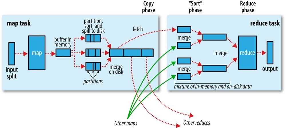
Figure 7-4. Shuffle and sort in MapReduce
Each map task has a circular memory buffer that it writes the output to. The buffer is 100 MB by default (the size can be tuned by changing the mapreduce.task.io.sort.mb property). When the contents of the buffer reach a certain threshold size
(mapreduce.map.sort.spill.percent, which has the default value 0.80, or 80%), a background thread will start to spill the contents to disk. Map outputs will continue to be written to the buffer while the spill takes place, but if the buffer fills up during this time, the map will block until the spill is complete. Spills are written in round-robin fashion to the directories specified by the mapreduce.cluster.local.dir property, in a job-specific subdirectory.
Before it writes to disk, the thread first divides the data into partitions corresponding to the reducers that they will ultimately be sent to. Within each partition, the background thread performs an in-memory sort by key, and if there is a combiner function, it is run on the output of the sort. Running the combiner function makes for a more compact map output, so there is less data to write to local disk and to transfer to the reducer.
Each time the memory buffer reaches the spill threshold, a new spill file is created, so after the map task has written its last output record, there could be several spill files. Before the task is finished, the spill files are merged into a single partitioned and sorted output file.
The configuration property mapreduce.task.io.sort.factor controls the maximum number of streams to merge at once; the default is 10.
If there are at least three spill files (set by the mapreduce.map.combine.minspills property), the combiner is run again before the output file is written. Recall that combiners may be run repeatedly over the input without affecting the final result. If there are only one or two spills, the potential reduction in map output size is not worth the overhead in invoking the combiner, so it is not run again for this map output.
It is often a good idea to compress the map output as it is written to disk, because doing so makes it faster to write to disk, saves disk space, and reduces the amount of data to transfer to the reducer. By default, the output is not compressed, but it is easy to enable this by setting mapreduce.map.output.compress to true. The compression library to use is specified by mapreduce.map.output.compress.codec; see Compression for more on compression formats.
The output file’s partitions are made available to the reducers over HTTP. The maximum number of worker threads used to serve the file partitions is controlled by the mapreduce.shuffle.max.threads property; this setting is per node manager, not per map task. The default of 0 sets the maximum number of threads to twice the number of processors on the machine.
The Reduce Side
Let’s turn now to the reduce part of the process. The map output file is sitting on the local disk of the machine that ran the map task (note that although map outputs always get written to local disk, reduce outputs may not be), but now it is needed by the machine that is about to run the reduce task for the partition. Moreover, the reduce task needs the map output for its particular partition from several map tasks across the cluster. The map tasks may finish at different times, so the reduce task starts copying their outputs as soon as each completes. This is known as the copy phase of the reduce task. The reduce task has a small number of copier threads so that it can fetch map outputs in parallel. The default is five threads, but this number can be changed by setting the mapreduce.reduce.shuffle.parallelcopies property.
NOTE
How do reducers know which machines to fetch map output from?
As map tasks complete successfully, they notify their application master using the heartbeat mechanism. Therefore, for a given job, the application master knows the mapping between map outputs and hosts. A thread in the reducer periodically asks the master for map output hosts until it has retrieved them all.
Hosts do not delete map outputs from disk as soon as the first reducer has retrieved them, as the reducer may subsequently fail. Instead, they wait until they are told to delete them by the application master, which is after the job has completed.
Map outputs are copied to the reduce task JVM’s memory if they are small enough (the buffer’s size is controlled by mapreduce.reduce.shuffle.input.buffer.percent, which specifies the proportion of the heap to use for this purpose); otherwise, they are copied to disk. When the in-memory buffer reaches a threshold size (controlled by mapreduce.reduce.shuffle.merge.percent) or reaches a threshold number of map outputs (mapreduce.reduce.merge.inmem.threshold), it is merged and spilled to disk. If a combiner is specified, it will be run during the merge to reduce the amount of data written to disk.
As the copies accumulate on disk, a background thread merges them into larger, sorted files. This saves some time merging later on. Note that any map outputs that were compressed (by the map task) have to be decompressed in memory in order to perform a merge on them.
When all the map outputs have been copied, the reduce task moves into the sort phase (which should properly be called the merge phase, as the sorting was carried out on the map side), which merges the map outputs, maintaining their sort ordering. This is done in rounds. For example, if there were 50 map outputs and the merge factor was 10 (the default, controlled by the mapreduce.task.io.sort.factor property, just like in the map’s merge), there would be five rounds. Each round would merge 10 files into 1, so at the end there would be 5 intermediate files.
Rather than have a final round that merges these five files into a single sorted file, the merge saves a trip to disk by directly feeding the reduce function in what is the last phase: the reduce phase. This final merge can come from a mixture of in-memory and on-disk segments.
NOTE
The number of files merged in each round is actually more subtle than this example suggests. The goal is to merge the minimum number of files to get to the merge factor for the final round. So if there were 40 files, the merge would not merge 10 files in each of the four rounds to get 4 files. Instead, the first round would merge only 4 files, and the subsequent three rounds would merge the full 10 files. The 4 merged files and the 6 (as yet unmerged) files make a total of 10 files for the final round. The process is illustrated in Figure 7-5.
Note that this does not change the number of rounds; it’s just an optimization to minimize the amount of data that is written to disk, since the final round always merges directly into the reduce.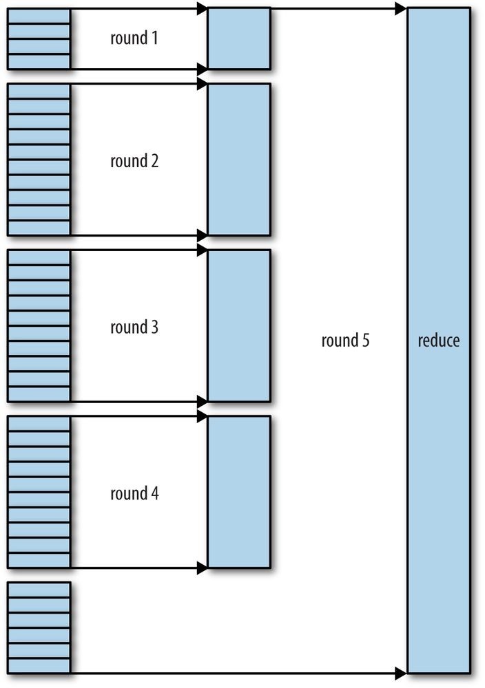
Figure 7-5. Efficiently merging 40 file segments with a merge factor of 10
During the reduce phase, the reduce function is invoked for each key in the sorted output.
The output of this phase is written directly to the output filesystem, typically HDFS. In the case of HDFS, because the node manager is also running a datanode, the first block replica will be written to the local disk.
Configuration Tuning
We are now in a better position to understand how to tune the shuffle to improve
MapReduce performance. The relevant settings, which can be used on a per-job basis (except where noted), are summarized in Tables 7-1 and 7-2, along with the defaults, which are good for general-purpose jobs.
The general principle is to give the shuffle as much memory as possible. However, there is a trade-off, in that you need to make sure that your map and reduce functions get enough memory to operate. This is why it is best to write your map and reduce functions to use as little memory as possible — certainly they should not use an unbounded amount of memory (avoid accumulating values in a map, for example).
The amount of memory given to the JVMs in which the map and reduce tasks run is set by the mapred.child.java.opts property. You should try to make this as large as possible for the amount of memory on your task nodes; the discussion in Memory settings in YARN and MapReduce goes through the constraints to consider.
On the map side, the best performance can be obtained by avoiding multiple spills to disk; one is optimal. If you can estimate the size of your map outputs, you can set the mapreduce.task.io.sort.* properties appropriately to minimize the number of spills. In particular, you should increase mapreduce.task.io.sort.mb if you can. There is a MapReduce counter (SPILLEDRECORDS; see Counters) that counts the total number of records that were spilled to disk over the course of a job, which can be useful for tuning. Note that the counter includes both map- and reduce-side spills.
On the reduce side, the best performance is obtained when the intermediate data can reside entirely in memory. This does not happen by default, since for the general case all the memory is reserved for the reduce function. But if your reduce function has light memory requirements, setting mapreduce.reduce.merge.inmem.threshold to 0 and mapreduce.reduce.input.buffer.percent to 1.0 (or a lower value; see Table 7-2) may bring a performance boost.
In April 2008, Hadoop won the general-purpose terabyte sort benchmark (as discussed in A Brief History of Apache Hadoop), and one of the optimizations used was keeping the intermediate data in memory on the reduce side.
More generally, Hadoop uses a buffer size of 4 KB by default, which is low, so you should increase this across the cluster (by setting io.file.buffer.size; see also Other Hadoop Properties).
_Table 7-1. Map-side tuning properties
Property name Type Default value Description
mapreduce.task.io.sort.mb int 100 The size, in
megabytes, of the memory
buffer to use
while sorting map output.
| mapreduce.map.sort.spill.percent | float | 0.80 | The threshold usage proportion for both the map output memory buffer and the record boundaries index to start the process of spilling to disk. |
|---|---|---|---|
mapreduce.task.io.sort.factor int 10 The
maximum number of streams to merge at once when sorting files. This property is also used in the reduce. It’s fairly
common to
increase this to 100.
| mapreduce.map.combine.minspills | int | 3 | The minimum number of spill files needed for the combiner to run (if a combiner is specified). |
|---|---|---|---|
mapreduce.map.output.compress boolean false Whether to
compress map outputs.
| mapreduce.map.output.compress.codec Class name | org.apache.hadoop.io.compress.DefaultCodec The compression codec to use for map outputs. |
|---|---|
mapreduce.shuffle.max.threads int 0 The number
of worker threads per node manager for serving the map outputs to reducers. This is a clusterwide setting and cannot be set by individual jobs. 0 means use the Netty default of twice the number of available processors.
Table 7-2. Reduce-side tuning properties
Property name Type Default Description
value
| mapreduce.reduce.shuffle.parallelcopies int 5 | The number of threads used to copy map outputs to the reducer. |
|---|---|
| mapreduce.reduce.shuffle.maxfetchfailures int 10 | The number of times a reducer tries to fetch a map output before reporting the error. |
| mapreduce.task.io.sort.factor int 10 | The maximum number of streams to merge at once when sorting files. This property is also used in the map. |
| mapreduce.reduce.shuffle.input.buffer.percent float 0.70 | The proportion of total heap size to be allocated to the map outputs buffer during the copy phase of the shuffle. |
mapreduce.reduce.shuffle.merge.percent float 0.66 The threshold usage proportion for the map
outputs buffer (defined by
mapred.job.shuffle.input.buffer.percent)
for starting the process of merging the outputs and spilling to disk.
| mapreduce.reduce.merge.inmem.threshold | int | 1000 | The threshold number of map outputs for starting the process of merging the outputs and spilling to disk. A value of 0 or less means there is no threshold, and the spill behavior is governed solely by mapreduce.reduce.shuffle.merge.percent. |
|---|---|---|---|
mapreduce.reduce.input.buffer.percent float 0.0 The proportion of total heap size to be used for
retaining map outputs in memory during the reduce. For the reduce phase to begin, the size of map outputs in memory must be no more than this size. By default, all map outputs are merged to disk before the reduce begins, to give the reducers as much memory as possible. However, if your reducers require less memory, this value may be increased to minimize the number of trips to disk.
Task Execution
We saw how the MapReduce system executes tasks in the context of the overall job at the beginning of this chapter, in Anatomy of a MapReduce Job Run. In this section, we’ll look at some more controls that MapReduce users have over task execution.
The Task Execution Environment
Hadoop provides information to a map or reduce task about the environment in which it is running. For example, a map task can discover the name of the file it is processing (see File information in the mapper), and a map or reduce task can find out the attempt number of the task. The properties in Table 7-3 can be accessed from the job’s configuration, obtained in the old MapReduce API by providing an implementation of the configure() method for Mapper or Reducer, where the configuration is passed in as an argument. In the new API, these properties can be accessed from the context object passed to all methods of the Mapper or Reducer.
Table 7-3. Task environment properties
| Property name Type | Description | Example |
|---|---|---|
| mapreduce.job.id String | The job ID (see Job, Task, and Task Attempt IDs for a description of the format) | job_200811201130_0004 |
| mapreduce.task.id String | The task ID | task_200811201130_0004_m_000003 |
| mapreduce.task.attempt.id String | The task attempt ID | attempt_200811201130_0004_m_000003_0 |
| mapreduce.task.partition int | The index of the task within the job | 3 |
| mapreduce.task.ismap boolean Whether this task is a map task | true |
Streaming environment variables
Hadoop sets job configuration parameters as environment variables for Streaming programs. However, it replaces nonalphanumeric characters with underscores to make sure they are valid names. The following Python expression illustrates how you can retrieve the value of the mapreduce.job.id property from within a Python Streaming script: os.environ[“mapreduce_job_id”]
You can also set environment variables for the Streaming processes launched by
MapReduce by supplying the -cmdenv option to the Streaming launcher program (once for each variable you wish to set). For example, the following sets the MAGIC_PARAMETER environment variable:
-cmdenv MAGIC_PARAMETER=abracadabra
Speculative Execution
The MapReduce model is to break jobs into tasks and run the tasks in parallel to make the overall job execution time smaller than it would be if the tasks ran sequentially. This makes the job execution time sensitive to slow-running tasks, as it takes only one slow task to make the whole job take significantly longer than it would have done otherwise.
When a job consists of hundreds or thousands of tasks, the possibility of a few straggling tasks is very real.
Tasks may be slow for various reasons, including hardware degradation or software misconfiguration, but the causes may be hard to detect because the tasks still complete successfully, albeit after a longer time than expected. Hadoop doesn’t try to diagnose and fix slow-running tasks; instead, it tries to detect when a task is running slower than expected and launches another equivalent task as a backup. This is termed speculative execution of tasks.
It’s important to understand that speculative execution does not work by launching two duplicate tasks at about the same time so they can race each other. This would be wasteful of cluster resources. Rather, the scheduler tracks the progress of all tasks of the same type
(map and reduce) in a job, and only launches speculative duplicates for the small proportion that are running significantly slower than the average. When a task completes successfully, any duplicate tasks that are running are killed since they are no longer needed. So, if the original task completes before the speculative task, the speculative task is killed; on the other hand, if the speculative task finishes first, the original is killed.
Speculative execution is an optimization, and not a feature to make jobs run more reliably. If there are bugs that sometimes cause a task to hang or slow down, relying on speculative execution to avoid these problems is unwise and won’t work reliably, since the same bugs are likely to affect the speculative task. You should fix the bug so that the task doesn’t hang or slow down.
Speculative execution is turned on by default. It can be enabled or disabled independently for map tasks and reduce tasks, on a cluster-wide basis, or on a per-job basis. The relevant properties are shown in Table 7-4.
Table 7-4. Speculative execution properties
Property name Type Default value
| mapreduce.map.speculative | boolean true |
|---|---|
| mapreduce.reduce.speculative boolean true |
yarn.app.mapreduce.am.job.speculator.class Class org.apache.hadoop.mapreduce.v2.app.speculate.
| yarn.app.mapreduce.am.job.task.estimator.class Class | org.apache.hadoop.mapreduce.v2.app.speculate. |
|---|---|
Why would you ever want to turn speculative execution off? The goal of speculative execution is to reduce job execution time, but this comes at the cost of cluster efficiency. On a busy cluster, speculative execution can reduce overall throughput, since redundant tasks are being executed in an attempt to bring down the execution time for a single job. For this reason, some cluster administrators prefer to turn it off on the cluster and have users explicitly turn it on for individual jobs. This was especially relevant for older versions of Hadoop, when speculative execution could be overly aggressive in scheduling speculative tasks.
There is a good case for turning off speculative execution for reduce tasks, since any duplicate reduce tasks have to fetch the same map outputs as the original task, and this can significantly increase network traffic on the cluster.
Another reason for turning off speculative execution is for nonidempotent tasks. However, in many cases it is possible to write tasks to be idempotent and use an OutputCommitter to promote the output to its final location when the task succeeds. This technique is explained in more detail in the next section.
Output Committers
Hadoop MapReduce uses a commit protocol to ensure that jobs and tasks either succeed or fail cleanly. The behavior is implemented by the OutputCommitter in use for the job, which is set in the old MapReduce API by calling the setOutputCommitter() on JobConf or by setting mapred.output.committer.class in the configuration. In the new MapReduce API, the OutputCommitter is determined by the OutputFormat, via its getOutputCommitter() method. The default is FileOutputCommitter, which is appropriate for file-based MapReduce. You can customize an existing OutputCommitter or even write a new implementation if you need to do special setup or cleanup for jobs or tasks.
The OutputCommitter API is as follows (in both the old and new MapReduce APIs):
public abstract class OutputCommitter {
public abstract void setupJob(JobContext jobContext) throws IOException; public void commitJob(JobContext jobContext) throws IOException { } public void abortJob(JobContext jobContext, JobStatus.State state) throws IOException { }
public abstract void setupTask(TaskAttemptContext taskContext) throws IOException; public abstract boolean needsTaskCommit(TaskAttemptContext taskContext) throws IOException; public abstract void commitTask(TaskAttemptContext taskContext) throws IOException; public abstract void abortTask(TaskAttemptContext taskContext) throws IOException;
} }
The setupJob() method is called before the job is run, and is typically used to perform initialization. For FileOutputCommitter, the method creates the final output directory, ${mapreduce.output.fileoutputformat.outputdir}, and a temporary working space for task output, temporary_, as a subdirectory underneath it.
If the job succeeds, the commitJob() method is called, which in the default file-based implementation deletes the temporary working space and creates a hidden empty marker file in the output directory called SUCCESS_ to indicate to filesystem clients that the job completed successfully. If the job did not succeed, abortJob() is called with a state object indicating whether the job failed or was killed (by a user, for example). In the default implementation, this will delete the job’s temporary working space.
The operations are similar at the task level. The setupTask() method is called before the task is run, and the default implementation doesn’t do anything, because temporary directories named for task outputs are created when the task outputs are written.
The commit phase for tasks is optional and may be disabled by returning false from needsTaskCommit(). This saves the framework from having to run the distributed commit protocol for the task, and neither commitTask() nor abortTask() is called.
FileOutputCommitter will skip the commit phase when no output has been written by a task.
If a task succeeds, commitTask() is called, which in the default implementation moves the temporary task output directory (which has the task attempt ID in its name to avoid conflicts between task attempts) to the final output path,
${mapreduce.output.fileoutputformat.outputdir}. Otherwise, the framework calls abortTask(), which deletes the temporary task output directory.
The framework ensures that in the event of multiple task attempts for a particular task, only one will be committed; the others will be aborted. This situation may arise because the first attempt failed for some reason — in which case, it would be aborted, and a later, successful attempt would be committed. It can also occur if two task attempts were running concurrently as speculative duplicates; in this instance, the one that finished first would be committed, and the other would be aborted.
Task side-effect files
The usual way of writing output from map and reduce tasks is by using OutputCollector to collect key-value pairs. Some applications need more flexibility than a single key-value pair model, so these applications write output files directly from the map or reduce task to a distributed filesystem, such as HDFS. (There are other ways to produce multiple outputs, too, as described in Multiple Outputs.)
Care needs to be taken to ensure that multiple instances of the same task don’t try to write to the same file. As we saw in the previous section, the OutputCommitter protocol solves this problem. If applications write side files in their tasks’ working directories, the side files for tasks that successfully complete will be promoted to the output directory automatically, whereas failed tasks will have their side files deleted.
A task may find its working directory by retrieving the value of the
mapreduce.task.output.dir property from the job configuration. Alternatively, a MapReduce program using the Java API may call the getWorkOutputPath() static method on FileOutputFormat to get the Path object representing the working directory. The framework creates the working directory before executing the task, so you don’t need to create it.
To take a simple example, imagine a program for converting image files from one format to another. One way to do this is to have a map-only job, where each map is given a set of images to convert (perhaps using NLineInputFormat; see NLineInputFormat). If a map task writes the converted images into its working directory, they will be promoted to the output directory when the task successfully finishes.
[51] In the old MapReduce API, you can call JobClient.submitJob(conf) or JobClient.runJob(conf).
[52] Not discussed in this section are the job history server daemon (for retaining job history data) and the shuffle handler auxiliary service (for serving map outputs to reduce tasks).
[53] If a Streaming process hangs, the node manager will kill it (along with the JVM that launched it) only in the following circumstances: either yarn.nodemanager.container-executor.class is set to org.apache.hadoop.yarn.server.nodemanager.LinuxContainerExecutor, or the default container executor is being used and the setsid command is available on the system (so that the task JVM and any processes it launches are in the same process group). In any other case, orphaned Streaming processes will accumulate on the system, which will impact utilization over time.
[54] The term shuffle is actually imprecise, since in some contexts it refers to only the part of the process where map outputs are fetched by reduce tasks. In this section, we take it to mean the whole process, from the point where a map produces output to where a reduce consumes input.

若有收获,就点个赞吧
0 人点赞
