- Chapter 8. MapReduce Types and Formats
- MapReduce Types
- Input Formats
- Output Formats
- Chapter 9. MapReduce Features
- Chapter 10. Setting Up a Hadoop Cluster
- Chapter 11. Administering Hadoop
- Chapter 12. Avro
- Chapter 13. Parquet
- Chapter 14. Flume
- Chapter 15. Sqoop
Chapter 8. MapReduce Types and Formats
MapReduce has a simple model of data processing: inputs and outputs for the map and reduce functions are key-value pairs. This chapter looks at the MapReduce model in detail, and in particular at how data in various formats, from simple text to structured binary objects, can be used with this model.
MapReduce Types
The map and reduce functions in Hadoop MapReduce have the following general form:
map: (K1, V1) → list(K2, V2) reduce: (K2, list(V2)) → list(K3, V3)
In general, the map input key and value types (K1 and V1) are different from the map output types (K2 and V2). However, the reduce input must have the same types as the map output, although the reduce output types may be different again (K3 and V3). The Java API mirrors this general form:
public class Mapper
// … }
protected void map(KEYIN key, VALUEIN value,
Context context) throws IOException, InterruptedException {
// …
} }
public class Reducer
// … }
protected void reduce(KEYIN key, Iterable
// …
} }
The context objects are used for emitting key-value pairs, and they are parameterized by the output types so that the signature of the write() method is:
public void write(KEYOUT key, VALUEOUT value) throws IOException, InterruptedException
Since Mapper and Reducer are separate classes, the type parameters have different scopes, and the actual type argument of KEYIN (say) in the Mapper may be different from the type of the type parameter of the same name (KEYIN) in the Reducer. For instance, in the maximum temperature example from earlier chapters, KEYIN is replaced by LongWritable for the Mapper and by Text for the Reducer.
Similarly, even though the map output types and the reduce input types must match, this is not enforced by the Java compiler.
The type parameters are named differently from the abstract types (KEYIN versus K1, and so on), but the form is the same.
If a combiner function is used, then it has the same form as the reduce function (and is an implementation of Reducer), except its output types are the intermediate key and value types (K2 and V2), so they can feed the reduce function:
map: (K1, V1) → list(K2, V2) combiner: (K2, list(V2)) → list(K2, V2) reduce: (K2, list(V2)) → list(K3, V3)
Often the combiner and reduce functions are the same, in which case K3 is the same as K2, and V3 is the same as V2.
The partition function operates on the intermediate key and value types (K2 and V2) and returns the partition index. In practice, the partition is determined solely by the key (the
value is ignored): partition: (K2, V2) → integer Or in Java:
public abstract class Partitioner
}
MAPREDUCE SIGNATURES IN THE OLD API In the old API (see Appendix D), the signatures are very similar and actually name the type parameters K1, V1, and so on, although the constraints on the types are exactly the same in both the old and new APIs:
public interface Mapper
OutputCollector
}
public interface Reducer
OutputCollector
}
public interface Partitioner
So much for the theory. How does this help you configure MapReduce jobs? Table 8-1 summarizes the configuration options for the new API (and Table 8-2 does the same for the old API). It is divided into the properties that determine the types and those that have to be compatible with the configured types.
Input types are set by the input format. So, for instance, a TextInputFormat generates keys of type LongWritable and values of type Text. The other types are set explicitly by calling the methods on the Job (or JobConf in the old API). If not set explicitly, the intermediate types default to the (final) output types, which default to LongWritable and Text. So, if K2 and K3 are the same, you don’t need to call setMapOutputKeyClass(), because it falls back to the type set by calling setOutputKeyClass(). Similarly, if V2 and V3 are the same, you only need to use setOutputValueClass().
It may seem strange that these methods for setting the intermediate and final output types exist at all. After all, why can’t the types be determined from a combination of the mapper and the reducer? The answer has to do with a limitation in Java generics: type erasure means that the type information isn’t always present at runtime, so Hadoop has to be given it explicitly. This also means that it’s possible to configure a MapReduce job with incompatible types, because the configuration isn’t checked at compile time. The settings that have to be compatible with the MapReduce types are listed in the lower part of Table 8-1. Type conflicts are detected at runtime during job execution, and for this reason, it is wise to run a test job using a small amount of data to flush out and fix any type incompatibilities.
Table 8-1. Configuration of MapReduce types in the new API
Property Job setter method Input Intermediate Output
types types types
| K1 | V1 | K2 | V2 | K3 | V3 | ||
|---|---|---|---|---|---|---|---|
| Properties for configuring types: | |||||||
| mapreduce.job.inputformat.class | setInputFormatClass() | • | • | ||||
| mapreduce.map.output.key.class | setMapOutputKeyClass() | • | |||||
| mapreduce.map.output.value.class | setMapOutputValueClass() | • | |||||
| mapreduce.job.output.key.class | setOutputKeyClass() | • | |||||
| mapreduce.job.output.value.class | setOutputValueClass() | • | |||||
| Properties that must be consistent with the types: | |||||||
| mapreduce.job.map.class setMapperClass() | • | • | • | • | |||
| mapreduce.job.combine.class setCombinerClass() | • | • | |||||
| mapreduce.job.partitioner.class setPartitionerClass() | • | • | |||||
| mapreduce.job.output.key.comparator.class setSortComparatorClass() | • | ||||||
| mapreduce.job.output.group.comparator.class setGroupingComparatorClass() | • | ||||||
| mapreduce.job.reduce.class setReducerClass() | • | • | • | • | |||
| mapreduce.job.outputformat.class setOutputFormatClass() | • | • |
Table 8-2. Configuration of MapReduce types in the old API
Property JobConf setter method Input Intermediate Output
types types types
| K1 | V1 | K2 | V2 | K3 | V3 | ||
|---|---|---|---|---|---|---|---|
| Properties for configuring types: | |||||||
| mapred.input.format.class | setInputFormat() | • | • | ||||
| mapred.mapoutput.key.class | setMapOutputKeyClass() | • | |||||
| mapred.mapoutput.value.class | setMapOutputValueClass() | • | |||||
| mapred.output.key.class | setOutputKeyClass() | • | |||||
| mapred.output.value.class | setOutputValueClass() | • | |||||
| Properties that must be consistent with | the types: | ||||||
| mapred.mapper.class | setMapperClass() | • | • | • | • | ||
| mapred.map.runner.class | setMapRunnerClass() | • | • | • | • | ||
| mapred.combiner.class | setCombinerClass() | • | • | ||||
| mapred.partitioner.class | setPartitionerClass() | • | • | ||||
| mapred.output.key.comparator.class | setOutputKeyComparatorClass() | • | |||||
| mapred.output.value.groupfn.class | setOutputValueGroupingComparator() | • | |||||
| mapred.reducer.class | setReducerClass() | • | • | • | • | ||
| mapred.output.format.class | setOutputFormat() | • | • |
The Default MapReduce Job
What happens when you run MapReduce without setting a mapper or a reducer? Let’s try it by running this minimal MapReduce program:
public class MinimalMapReduce extends Configured implements Tool {
@Override
public int run(String[] args) throws Exception { if (args.length != 2) {
System.err.printf(“Usage: %s [generic options]
Example 8-1. A minimal MapReduce driver, with the defaults explicitly set
public class MinimalMapReduceWithDefaults extends Configured implements Tool {
@Override
public int run(String[] args) throws Exception {
Job job = JobBuilder.parseInputAndOutput(this, getConf(), args); if (job == null) { return -1;
} job.setInputFormatClass(TextInputFormat.class);
job.setMapperClass(Mapper.class);
job.setMapOutputKeyClass(LongWritable.class); job.setMapOutputValueClass(Text.class);
job.setPartitionerClass(HashPartitioner.class);
job.setNumReduceTasks(1); job.setReducerClass(Reducer.class); job.setOutputKeyClass(LongWritable.class); job.setOutputValueClass(Text.class);
job.setOutputFormatClass(TextOutputFormat.class);
return job.waitForCompletion(true) ? 0 : 1;
}
public static void main(String[] args) throws Exception { int exitCode = ToolRunner.run(new MinimalMapReduceWithDefaults(), args);
System.exit(exitCode);
} }
We’ve simplified the first few lines of the run() method by extracting the logic for printing usage and setting the input and output paths into a helper method. Almost all MapReduce drivers take these two arguments (input and output), so reducing the boilerplate code here is a good thing. Here are the relevant methods in the JobBuilder class for reference:
public static Job parseInputAndOutput(Tool tool, Configuration conf,
String[] args) throws IOException {
if (args.length != 2) { printUsage(tool, “
The default Streaming job
In Streaming, the default job is similar, but not identical, to the Java equivalent. The basic form is:
% hadoop jar $HADOOP_HOME/share/hadoop/tools/lib/hadoop-streaming-*.jar \ -input input/ncdc/sample.txt \
-output output \
-mapper /bin/cat
When we specify a non-Java mapper and the default text mode is in effect (-io text), Streaming does something special. It doesn’t pass the key to the mapper process; it just passes the value. (For other input formats, the same effect can be achieved by setting stream.map.input.ignoreKey to true.) This is actually very useful because the key is just the line offset in the file and the value is the line, which is all most applications are interested in. The overall effect of this job is to perform a sort of the input.
With more of the defaults spelled out, the command looks like this (notice that Streaming uses the old MapReduce API classes):
% hadoop jar $HADOOP_HOME/share/hadoop/tools/lib/hadoop-streaming-*.jar \
-input input/ncdc/sample.txt \
-output output \
-inputformat org.apache.hadoop.mapred.TextInputFormat \
-mapper /bin/cat \
-partitioner org.apache.hadoop.mapred.lib.HashPartitioner \
-numReduceTasks 1 \
-reducer org.apache.hadoop.mapred.lib.IdentityReducer \
-outputformat org.apache.hadoop.mapred.TextOutputFormat -io text
The -mapper and -reducer arguments take a command or a Java class. A combiner may optionally be specified using the -combiner argument.
Keys and values in Streaming
A Streaming application can control the separator that is used when a key-value pair is turned into a series of bytes and sent to the map or reduce process over standard input. The default is a tab character, but it is useful to be able to change it in the case that the keys or values themselves contain tab characters.
Similarly, when the map or reduce writes out key-value pairs, they may be separated by a configurable separator. Furthermore, the key from the output can be composed of more than the first field: it can be made up of the first n fields (defined by stream.num.map.output.key.fields or stream.num.reduce.output.key.fields), with the value being the remaining fields. For example, if the output from a Streaming process was a,b,c (with a comma as the separator), and n was 2, the key would be parsed as a,b and the value as c.
Separators may be configured independently for maps and reduces. The properties are listed in Table 8-3 and shown in a diagram of the data flow path in Figure 8-1.
These settings do not have any bearing on the input and output formats. For example, if stream.reduce.output.field.separator were set to be a colon, say, and the reduce stream process wrote the line a:b to standard out, the Streaming reducer would know to extract the key as a and the value as b. With the standard TextOutputFormat, this record would be written to the output file with a tab separating a and b. You can change the separator that TextOutputFormat uses by setting mapreduce.output.textoutputformat.separator.
Table 8-3. Streaming separator properties
Property name Type Default Description
value
| stream.map.input.field.separator | String | \t | The separator to use when passing the input key and value strings to the stream map process as a stream of bytes |
|---|---|---|---|
| stream.map.output.field.separator | String | \t | The separator to use when splitting the output from the stream map process into key and value strings for the map output |
| stream.num.map.output.key.fields | int | 1 | The number of fields separated by stream.map.output.field.separator to treat as the map output key |
| stream.reduce.input.field.separator | String | \t | The separator to use when passing the input key and value strings to the stream reduce process as a stream of bytes |
| stream.reduce.output.field.separator String | \t | The separator to use when splitting the output from the stream reduce process into key and value strings for the final reduce output | |
| stream.num.reduce.output.key.fields int | 1 | The number of fields separated by stream.reduce.output.field.separator to treat as the reduce output key |
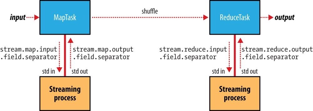
Figure 8-1. Where separators are used in a Streaming MapReduce job
Input Formats
Hadoop can process many different types of data formats, from flat text files to databases. In this section, we explore the different formats available.
Input Splits and Records
As we saw in Chapter 2, an input split is a chunk of the input that is processed by a single map. Each map processes a single split. Each split is divided into records, and the map processes each record — a key-value pair — in turn. Splits and records are logical: there is nothing that requires them to be tied to files, for example, although in their most common incarnations, they are. In a database context, a split might correspond to a range of rows from a table and a record to a row in that range (this is precisely the case with DBInputFormat, which is an input format for reading data from a relational database).
Input splits are represented by the Java class InputSplit (which, like all of the classes mentioned in this section, is in the org.apache.hadoop.mapreduce package):55]
public abstract class InputSplit { public abstract long getLength() throws IOException, InterruptedException; public abstract String[] getLocations() throws IOException,
InterruptedException;
}
An InputSplit has a length in bytes and a set of storage locations, which are just hostname strings. Notice that a split doesn’t contain the input data; it is just a reference to the data. The storage locations are used by the MapReduce system to place map tasks as close to the split’s data as possible, and the size is used to order the splits so that the largest get processed first, in an attempt to minimize the job runtime (this is an instance of a greedy approximation algorithm).
As a MapReduce application writer, you don’t need to deal with InputSplits directly, as they are created by an InputFormat (an InputFormat is responsible for creating the input splits and dividing them into records). Before we see some concrete examples of
InputFormats, let’s briefly examine how it is used in MapReduce. Here’s the interface:
public abstract class InputFormat
public abstract RecordReader
The client running the job calculates the splits for the job by calling getSplits(), then sends them to the application master, which uses their storage locations to schedule map tasks that will process them on the cluster. The map task passes the split to the createRecordReader() method on InputFormat to obtain a RecordReader for that split. A RecordReader is little more than an iterator over records, and the map task uses one to generate record key-value pairs, which it passes to the map function. We can see this by looking at the Mapper’s run() method:
public void run(Context context) throws IOException, InterruptedException { setup(context);
while (context.nextKeyValue()) { map(context.getCurrentKey(), context.getCurrentValue(), context);
}
cleanup(context); }
After running setup(), the nextKeyValue() is called repeatedly on the Context (which delegates to the identically named method on the RecordReader) to populate the key and value objects for the mapper. The key and value are retrieved from the RecordReader by way of the Context and are passed to the map() method for it to do its work. When the reader gets to the end of the stream, the nextKeyValue() method returns false, and the map task runs its cleanup() method and then completes.
WARNING Although it’s not shown in the code snippet, for reasons of efficiency, RecordReader implementations will return the same key and value objects on each call to getCurrentKey() and getCurrentValue(). Only the contents of these objects are changed by the reader’s nextKeyValue() method. This can be a surprise to users, who might expect keys and values to be immutable and not to be reused. This causes problems when a reference to a key or value object is retained outside the map() method, as its value can change without warning. If you need to do this, make a copy of the object you want to hold on to. For example, for a Text object, you can use its copy constructor: new Text(value).
The situation is similar with reducers. In this case, the value objects in the reducer’s iterator are reused, so you need to copy any that you need to retain between calls to the iterator (see Example 9-11).
Finally, note that the Mapper’s run() method is public and may be customized by users. MultithreadedMapper is an implementation that runs mappers concurrently in a configurable number of threads (set by mapreduce.mapper.multithreadedmapper.threads). For most data processing tasks, it confers no advantage over the default implementation. However, for mappers that spend a long time processing each record — because they contact external servers, for example — it allows multiple mappers to run in one JVM with little contention.
FileInputFormat
FileInputFormat is the base class for all implementations of InputFormat that use files as their data source (see Figure 8-2). It provides two things: a place to define which files are included as the input to a job, and an implementation for generating splits for the input files. The job of dividing splits into records is performed by subclasses.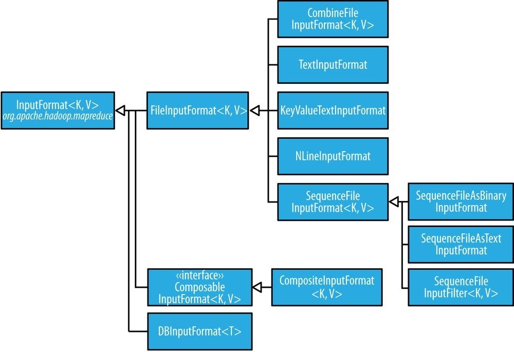
Figure 8-2. InputFormat class hierarchy
FileInputFormat input paths
The input to a job is specified as a collection of paths, which offers great flexibility in constraining the input. FileInputFormat offers four static convenience methods for setting a Job’s input paths:
public static void addInputPath(Job job, Path path) public static void addInputPaths(Job job, String commaSeparatedPaths) public static void setInputPaths(Job job, Path… inputPaths) public static void setInputPaths(Job job, String commaSeparatedPaths)
The addInputPath() and addInputPaths() methods add a path or paths to the list of inputs. You can call these methods repeatedly to build the list of paths. The setInputPaths() methods set the entire list of paths in one go (replacing any paths set on the Job in previous calls).
A path may represent a file, a directory, or, by using a glob, a collection of files and directories. A path representing a directory includes all the files in the directory as input to the job. See File patterns for more on using globs.
WARNING The contents of a directory specified as an input path are not processed recursively. In fact, the directory should only contain files. If the directory contains a subdirectory, it will be interpreted as a file, which will cause an error. The way to handle this case is to use a file glob or a filter to select only the files in the directory based on a name pattern.
Alternatively, mapreduce.input.fileinputformat.input.dir.recursive can be set to true to force the input directory to be read recursively.
The add and set methods allow files to be specified by inclusion only. To exclude certain files from the input, you can set a filter using the setInputPathFilter() method on FileInputFormat. Filters are discussed in more detail in PathFilter.
Even if you don’t set a filter, FileInputFormat uses a default filter that excludes hidden files (those whose names begin with a dot or an underscore). If you set a filter by calling setInputPathFilter(), it acts in addition to the default filter. In other words, only nonhidden files that are accepted by your filter get through.
Paths and filters can be set through configuration properties, too (Table 8-4), which can be handy for Streaming jobs. Setting paths is done with the -input option for the Streaming interface, so setting paths directly usually is not needed.
Table 8-4. Input path and filter properties
Property name Type Default Description value
| mapreduce.input.fileinputformat.inputdir Comma- None separated paths |
The input files for a job. Paths that contain commas should have those commas escaped by a backslash character. For example, the glob {a,b} would be escaped as {a\,b}. |
|---|---|
| mapreduce.input.pathFilter.class PathFilter None classname | The filter to apply to the input files for a job. |
FileInputFormat input splits
Given a set of files, how does FileInputFormat turn them into splits? FileInputFormat splits only large files — here, “large” means larger than an HDFS block. The split size is normally the size of an HDFS block, which is appropriate for most applications; however, it is possible to control this value by setting various Hadoop properties, as shown in Table 8-5.
Table 8-5. Properties for controlling split size
Property name Type Default value Description
| mapreduce.input.fileinputformat.split.minsize int | 1 | The smallest valid size in bytes for a file split |
|---|---|---|
| mapreduce.input.fileinputformat.split.maxsize long [a] |
Long.MAX_VALUE (i.e., 9223372036854775807) | The largest valid size in bytes for a file split |
| dfs.blocksize long | 128 MB (i.e., 134217728) | The size of a block in HDFS in bytes |
[a] This property is not present in the old MapReduce API (with the exception of CombineFileInputFormat). Instead, it is calculated indirectly as the size of the total input for the job, divided by the guide number of map tasks specified by mapreduce.job.maps (or the setNumMapTasks() method on JobConf). Because the number of map tasks defaults to 1, this makes the maximum split size the size of the input.
The minimum split size is usually 1 byte, although some formats have a lower bound on the split size. (For example, sequence files insert sync entries every so often in the stream, so the minimum split size has to be large enough to ensure that every split has a sync point to allow the reader to resynchronize with a record boundary. See Reading a SequenceFile.)
Applications may impose a minimum split size. By setting this to a value larger than the block size, they can force splits to be larger than a block. There is no good reason for doing this when using HDFS, because doing so will increase the number of blocks that are not local to a map task.
The maximum split size defaults to the maximum value that can be represented by a Java long type. It has an effect only when it is less than the block size, forcing splits to be smaller than a block.
The split size is calculated by the following formula (see the computeSplitSize() method in FileInputFormat):
max(minimumSize, min(maximumSize, blockSize))
and by default: minimumSize < blockSize < maximumSize
so the split size is blockSize. Various settings for these parameters and how they affect the final split size are illustrated in Table 8-6.
Table 8-6. Examples of how to control the split size
Minimum Maximum split Block Split Comment
| split size | size | size | size | |
|---|---|---|---|---|
| 1 (default) |
Long.MAX_VALUE (default) |
128 MB (default) |
128 MB |
By default, the split size is the same as the default block size. |
| 1 (default) |
Long.MAX_VALUE (default) |
256 MB | 256 MB |
The most natural way to increase the split size is to have larger blocks in HDFS, either by setting dfs.blocksize or by configuring this on a perfile basis at file construction time. |
| 256 MB | Long.MAX_VALUE (default) |
128 MB (default) |
256 MB |
Making the minimum split size greater than the block size increases the split size, but at the cost of locality. |
| 1 (default) |
64 MB | 128 MB (default) |
64 MB |
Making the maximum split size less than the block size decreases the split size. |
Small files and CombineFileInputFormat
Hadoop works better with a small number of large files than a large number of small files. One reason for this is that FileInputFormat generates splits in such a way that each split is all or part of a single file. If the file is very small (“small” means significantly smaller than an HDFS block) and there are a lot of them, each map task will process very little input, and there will be a lot of them (one per file), each of which imposes extra bookkeeping overhead. Compare a 1 GB file broken into eight 128 MB blocks with 10,000 or so 100 KB files. The 10,000 files use one map each, and the job time can be tens or hundreds of times slower than the equivalent one with a single input file and eight map tasks.
The situation is alleviated somewhat by CombineFileInputFormat, which was designed to
work well with small files. Where FileInputFormat creates a split per file,
CombineFileInputFormat packs many files into each split so that each mapper has more to process. Crucially, CombineFileInputFormat takes node and rack locality into account when deciding which blocks to place in the same split, so it does not compromise the speed at which it can process the input in a typical MapReduce job.
Of course, if possible, it is still a good idea to avoid the many small files case, because
MapReduce works best when it can operate at the transfer rate of the disks in the cluster, and processing many small files increases the number of seeks that are needed to run a job. Also, storing large numbers of small files in HDFS is wasteful of the namenode’s memory. One technique for avoiding the many small files case is to merge small files into larger files by using a sequence file, as in Example 8-4; with this approach, the keys can act as filenames (or a constant such as NullWritable, if not needed) and the values as file contents. But if you already have a large number of small files in HDFS, then CombineFileInputFormat is worth trying.
NOTE CombineFileInputFormat isn’t just good for small files. It can bring benefits when processing large files, too, since it will generate one split per node, which may be made up of multiple blocks. Essentially, CombineFileInputFormat decouples the amount of data that a mapper consumes from the block size of the files in HDFS.
Preventing splitting
Some applications don’t want files to be split, as this allows a single mapper to process each input file in its entirety. For example, a simple way to check if all the records in a file are sorted is to go through the records in order, checking whether each record is not less than the preceding one. Implemented as a map task, this algorithm will work only if one map processes the whole file.56]
There are a couple of ways to ensure that an existing file is not split. The first (quick-anddirty) way is to increase the minimum split size to be larger than the largest file in your system. Setting it to its maximum value, Long.MAX_VALUE, has this effect. The second is to subclass the concrete subclass of FileInputFormat that you want to use, to override the isSplitable() method57] to return false. For example, here’s a nonsplittable TextInputFormat:
import org.apache.hadoop.fs.Path;
import org.apache.hadoop.mapreduce.JobContext;
import org.apache.hadoop.mapreduce.lib.input.TextInputFormat;
public class NonSplittableTextInputFormat extends TextInputFormat {
@Override
protected boolean isSplitable(JobContext context, Path file) { return false;
}
}
File information in the mapper
A mapper processing a file input split can find information about the split by calling the getInputSplit() method on the Mapper’s Context object. When the input format derives from FileInputFormat, the InputSplit returned by this method can be cast to a FileSplit to access the file information listed in Table 8-7.
In the old MapReduce API, and the Streaming interface, the same file split information is made available through properties that can be read from the mapper’s configuration. (In the old MapReduce API this is achieved by implementing configure() in your Mapper implementation to get access to the JobConf object.)
In addition to the properties in Table 8-7, all mappers and reducers have access to the properties listed in The Task Execution Environment.
Table 8-7. File split properties
| FileSplit method | Property name | Type Description |
|---|---|---|
| getPath() | mapreduce.map.input.file | Path/String The path of the input file being processed |
| getStart() | mapreduce.map.input.start | long The byte offset of the start of the split from the beginning of the file |
| getLength() | mapreduce.map.input.length | long The length of the split in bytes |
In the next section, we’ll see how to use a FileSplit when we need to access the split’s filename.
Processing a whole file as a record
A related requirement that sometimes crops up is for mappers to have access to the full contents of a file. Not splitting the file gets you part of the way there, but you also need to have a RecordReader that delivers the file contents as the value of the record. The listing for WholeFileInputFormat in Example 8-2 shows a way of doing this. Example 8-2. An InputFormat for reading a whole file as a record
public class WholeFileInputFormat extends FileInputFormat
@Override
protected boolean isSplitable(JobContext context, Path file) { return false; }
@Override
public RecordReader
InputSplit split, TaskAttemptContext context) throws IOException,
InterruptedException {
WholeFileRecordReader reader = new WholeFileRecordReader(); reader.initialize(split, context); return reader;
} }
WholeFileInputFormat defines a format where the keys are not used, represented by NullWritable, and the values are the file contents, represented by BytesWritable instances. It defines two methods. First, the format is careful to specify that input files should never be split, by overriding isSplitable() to return false. Second, we implement createRecordReader() to return a custom implementation of RecordReader, which appears in Example 8-3.
Example 8-3. The RecordReader used by WholeFileInputFormat for reading a whole file as a record
class WholeFileRecordReader extends RecordReader
private FileSplit fileSplit; private Configuration conf; private BytesWritable value = new BytesWritable(); private boolean processed = false;
@Override
public void initialize(InputSplit split, TaskAttemptContext context) throws IOException, InterruptedException { this.fileSplit = (FileSplit) split; this.conf = context.getConfiguration(); }
@Override
public boolean nextKeyValue() throws IOException, InterruptedException { if (!processed) {
byte[] contents = new byte[(int) fileSplit.getLength()];
Path file = fileSplit.getPath();
FileSystem fs = file.getFileSystem(conf);
FSDataInputStream in = null; try { in = fs.open(file);
IOUtils.readFully(in, contents, 0, contents.length); value.set(contents, 0, contents.length);
} finally {
IOUtils.closeStream(in);
}
processed = true; return true;
}
return false;
}
@Override
public NullWritable getCurrentKey() throws IOException, InterruptedException { return NullWritable.get(); }
@Override
public BytesWritable getCurrentValue() throws IOException, InterruptedException { return value; }
@Override
public float getProgress() throws IOException { return processed ? 1.0f : 0.0f; }
@Override
public void close() throws IOException {
// do nothing
} }
WholeFileRecordReader is responsible for taking a FileSplit and converting it into a single record, with a null key and a value containing the bytes of the file. Because there is only a single record, WholeFileRecordReader has either processed it or not, so it maintains a Boolean called processed. If the file has not been processed when the nextKeyValue() method is called, then we open the file, create a byte array whose length is the length of the file, and use the Hadoop IOUtils class to slurp the file into the byte array. Then we set the array on the BytesWritable instance that was passed into the next() method, and return true to signal that a record has been read.
The other methods are straightforward bookkeeping methods for accessing the current key and value types and getting the progress of the reader, and a close() method, which is invoked by the MapReduce framework when the reader is done.
To demonstrate how WholeFileInputFormat can be used, consider a MapReduce job for packaging small files into sequence files, where the key is the original filename and the value is the content of the file. The listing is in Example 8-4.
Example 8-4. A MapReduce program for packaging a collection of small files as a single SequenceFile
public class SmallFilesToSequenceFileConverter extends Configured implements Tool {
static class SequenceFileMapper
extends Mapper
private Text filenameKey;
@Override
protected void setup(Context context) throws IOException,
InterruptedException {
InputSplit split = context.getInputSplit(); Path path = ((FileSplit) split).getPath(); filenameKey = new Text(path.toString());
}
@Override
protected void map(NullWritable key, BytesWritable value, Context context) throws IOException, InterruptedException { context.write(filenameKey, value);
}
}
@Override
public int run(String[] args) throws Exception {
Job job = JobBuilder.parseInputAndOutput(this, getConf(), args); if (job == null) { return -1;
}
job.setInputFormatClass(WholeFileInputFormat.class); job.setOutputFormatClass(SequenceFileOutputFormat.class);
job.setOutputKeyClass(Text.class); job.setOutputValueClass(BytesWritable.class); job.setMapperClass(SequenceFileMapper.class);
return job.waitForCompletion(true) ? 0 : 1;
}
public static void main(String[] args) throws Exception { int exitCode = ToolRunner.run(new SmallFilesToSequenceFileConverter(), args);
System.exit(exitCode);
} }
Because the input format is a WholeFileInputFormat, the mapper only has to find the filename for the input file split. It does this by casting the InputSplit from the context to a FileSplit, which has a method to retrieve the file path. The path is stored in a Text object for the key. The reducer is the identity (not explicitly set), and the output format is a SequenceFileOutputFormat.
Here’s a run on a few small files. We’ve chosen to use two reducers, so we get two output sequence files:
% hadoop jar hadoop-examples.jar SmallFilesToSequenceFileConverter \ -conf conf/hadoop-localhost.xml -D mapreduce.job.reduces=2 \ input/smallfiles output
Two part files are created, each of which is a sequence file. We can inspect these with the -text option to the filesystem shell:
% hadoop fs -conf conf/hadoop-localhost.xml -text output/part-r-00000 hdfs://localhost/user/tom/input/smallfiles/a 61 61 61 61 61 61 61 61 61 61 hdfs://localhost/user/tom/input/smallfiles/c 63 63 63 63 63 63 63 63 63 63 hdfs://localhost/user/tom/input/smallfiles/e
% hadoop fs -conf conf/hadoop-localhost.xml -text output/part-r-00001 hdfs://localhost/user/tom/input/smallfiles/b 62 62 62 62 62 62 62 62 62 62 hdfs://localhost/user/tom/input/smallfiles/d 64 64 64 64 64 64 64 64 64 64 hdfs://localhost/user/tom/input/smallfiles/f 66 66 66 66 66 66 66 66 66 66
The input files were named a, b, c, d, e, and f, and each contained 10 characters of the corresponding letter (so, for example, a contained 10 “a” characters), except e, which was empty. We can see this in the textual rendering of the sequence files, which prints the filename followed by the hex representation of the file.
TIP There’s at least one way we could improve this program. As mentioned earlier, having one mapper per file is inefficient, so subclassing CombineFileInputFormat instead of FileInputFormat would be a better approach.
Text Input
Hadoop excels at processing unstructured text. In this section, we discuss the different InputFormats that Hadoop provides to process text.
TextInputFormat
TextInputFormat is the default InputFormat. Each record is a line of input. The key, a LongWritable, is the byte offset within the file of the beginning of the line. The value is the contents of the line, excluding any line terminators (e.g., newline or carriage return), and is packaged as a Text object. So, a file containing the following text:
On the top of the Crumpetty Tree
The Quangle Wangle sat, But his face you could not see, On account of his Beaver Hat. is divided into one split of four records. The records are interpreted as the following keyvalue pairs:
(0, On the top of the Crumpetty Tree) (33, The Quangle Wangle sat,)
(57, But his face you could not see,)
(89, On account of his Beaver Hat.)
Clearly, the keys are not line numbers. This would be impossible to implement in general, in that a file is broken into splits at byte, not line, boundaries. Splits are processed independently. Line numbers are really a sequential notion. You have to keep a count of lines as you consume them, so knowing the line number within a split would be possible, but not within the file.
However, the offset within the file of each line is known by each split independently of the other splits, since each split knows the size of the preceding splits and just adds this onto the offsets within the split to produce a global file offset. The offset is usually sufficient for applications that need a unique identifier for each line. Combined with the file’s name, it is unique within the filesystem. Of course, if all the lines are a fixed width, calculating the line number is simply a matter of dividing the offset by the width.
THE RELATIONSHIP BETWEEN INPUT SPLITS AND HDFS BLOCKS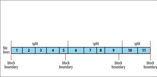 The logical records that FileInputFormats define usually do not fit neatly into HDFS blocks. For example, a TextInputFormat’s logical records are lines, which will cross HDFS boundaries more often than not. This has no bearing on the functioning of your program — lines are not missed or broken, for example — but it’s worth knowing about because it does mean that data-local maps (that is, maps that are running on the same host as their input data) will perform some remote reads. The slight overhead this causes is not normally significant.
Figure 8-3 shows an example. A single file is broken into lines, and the line boundaries do not correspond with the HDFS block boundaries. Splits honor logical record boundaries (in this case, lines), so we see that the first split contains line 5, even though it spans the first and second block. The second split starts at line 6.
Figure 8-3. Logical records and HDFS blocks for TextInputFormat
Controlling the maximum line length
If you are using one of the text input formats discussed here, you can set a maximum expected line length to safeguard against corrupted files. Corruption in a file can manifest itself as a very long line, which can cause out-of-memory errors and then task failure. By setting mapreduce.input.linerecordreader.line.maxlength to a value in bytes that fits in memory (and is comfortably greater than the length of lines in your input data), you ensure that the record reader will skip the (long) corrupt lines without the task failing.
KeyValueTextInputFormat
TextInputFormat’s keys, being simply the offsets within the file, are not normally very useful. It is common for each line in a file to be a key-value pair, separated by a delimiter such as a tab character. For example, this is the kind of output produced by
TextOutputFormat, Hadoop’s default OutputFormat. To interpret such files correctly, KeyValueTextInputFormat is appropriate. You can specify the separator via the
mapreduce.input.keyvaluelinerecordreader.key.value.separator property. It is a tab character by default. Consider the following input file, where → represents a (horizontal) tab character:
line1→On the top of the Crumpetty Tree line2→The Quangle Wangle sat, line3→But his face you could not see, line4→On account of his Beaver Hat.
Like in the TextInputFormat case, the input is in a single split comprising four records, although this time the keys are the Text sequences before the tab in each line:
(line1, On the top of the Crumpetty Tree)
(line2, The Quangle Wangle sat,)
(line3, But his face you could not see,)
(line4, On account of his Beaver Hat.)
NLineInputFormat
With TextInputFormat and KeyValueTextInputFormat, each mapper receives a variable number of lines of input. The number depends on the size of the split and the length of the lines. If you want your mappers to receive a fixed number of lines of input, then
NLineInputFormat is the InputFormat to use. Like with TextInputFormat, the keys are the byte offsets within the file and the values are the lines themselves.
N refers to the number of lines of input that each mapper receives. With N set to 1 (the default), each mapper receives exactly one line of input. The mapreduce.input.lineinputformat.linespermap property controls the value of N. By way of example, consider these four lines again:
On the top of the Crumpetty Tree
The Quangle Wangle sat, But his face you could not see, On account of his Beaver Hat.
If, for example, N is 2, then each split contains two lines. One mapper will receive the first two key-value pairs:
(0, On the top of the Crumpetty Tree)
(33, The Quangle Wangle sat,)
And another mapper will receive the second two key-value pairs:
(57, But his face you could not see,)
(89, On account of his Beaver Hat.)
The keys and values are the same as those that TextInputFormat produces. The difference is in the way the splits are constructed.
Usually, having a map task for a small number of lines of input is inefficient (due to the overhead in task setup), but there are applications that take a small amount of input data and run an extensive (i.e., CPU-intensive) computation for it, then emit their output. Simulations are a good example. By creating an input file that specifies input parameters, one per line, you can perform a parameter sweep: run a set of simulations in parallel to find how a model varies as the parameter changes.
WARNING If you have long-running simulations, you may fall afoul of task timeouts. When a task doesn’t report progress for more than 10 minutes, the application master assumes it has failed and aborts the process (see Task Failure).
The best way to guard against this is to report progress periodically, by writing a status message or incrementing a counter, for example. See What Constitutes Progress in MapReduce?.
Another example is using Hadoop to bootstrap data loading from multiple data sources, such as databases. You create a “seed” input file that lists the data sources, one per line. Then each mapper is allocated a single data source, and it loads the data from that source into HDFS. The job doesn’t need the reduce phase, so the number of reducers should be set to zero (by calling setNumReduceTasks() on Job). Furthermore, MapReduce jobs can be run to process the data loaded into HDFS. See Appendix C for an example.
XML
Most XML parsers operate on whole XML documents, so if a large XML document is made up of multiple input splits, it is a challenge to parse these individually. Of course, you can process the entire XML document in one mapper (if it is not too large) using the technique in Processing a whole file as a record.
Large XML documents that are composed of a series of “records” (XML document fragments) can be broken into these records using simple string or regular-expression matching to find the start and end tags of records. This alleviates the problem when the document is split by the framework because the next start tag of a record is easy to find by simply scanning from the start of the split, just like TextInputFormat finds newline boundaries.
Hadoop comes with a class for this purpose called StreamXmlRecordReader (which is in the org.apache.hadoop.streaming.mapreduce package, although it can be used outside of Streaming). You can use it by setting your input format to StreamInputFormat and setting the stream.recordreader.class property to org.apache.hadoop.streaming.mapreduce.StreamXmlRecordReader. The reader is
configured by setting job configuration properties to tell it the patterns for the start and end tags (see the class documentation for details).58]
To take an example, Wikipedia provides dumps of its content in XML form, which are appropriate for processing in parallel with MapReduce using this approach. The data is contained in one large XML wrapper document, which contains a series of elements, such as page elements that contain a page’s content and associated metadata. Using
StreamXmlRecordReader, the page elements can be interpreted as records for processing by a mapper.
Binary Input
Hadoop MapReduce is not restricted to processing textual data. It has support for binary formats, too.
SequenceFileInputFormat
Hadoop’s sequence file format stores sequences of binary key-value pairs. Sequence files are well suited as a format for MapReduce data because they are splittable (they have sync points so that readers can synchronize with record boundaries from an arbitrary point in the file, such as the start of a split), they support compression as a part of the format, and they can store arbitrary types using a variety of serialization frameworks. (These topics are covered in SequenceFile.)
To use data from sequence files as the input to MapReduce, you can use
SequenceFileInputFormat. The keys and values are determined by the sequence file, and you need to make sure that your map input types correspond. For example, if your sequence file has IntWritable keys and Text values, like the one created in Chapter 5, then the map signature would be Mapper
NOTE Although its name doesn’t give it away, SequenceFileInputFormat can read map files as well as sequence files. If it finds a directory where it was expecting a sequence file, SequenceFileInputFormat assumes that it is reading a map file and uses its datafile. This is why there is no MapFileInputFormat class.
SequenceFileAsTextInputFormat
SequenceFileAsTextInputFormat is a variant of SequenceFileInputFormat that converts
the sequence file’s keys and values to Text objects. The conversion is performed by calling toString() on the keys and values. This format makes sequence files suitable input for Streaming.
SequenceFileAsBinaryInputFormat
SequenceFileAsBinaryInputFormat is a variant of SequenceFileInputFormat that retrieves the sequence file’s keys and values as opaque binary objects. They are encapsulated as BytesWritable objects, and the application is free to interpret the underlying byte array as it pleases. In combination with a process that creates sequence files with SequenceFile.Writer’s appendRaw() method or
SequenceFileAsBinaryOutputFormat, this provides a way to use any binary data types with MapReduce (packaged as a sequence file), although plugging into Hadoop’s serialization mechanism is normally a cleaner alternative (see Serialization Frameworks).
FixedLengthInputFormat
FixedLengthInputFormat is for reading fixed-width binary records from a file, when the records are not separated by delimiters. The record size must be set via fixedlengthinputformat.record.length. Multiple Inputs
Although the input to a MapReduce job may consist of multiple input files (constructed by a combination of file globs, filters, and plain paths), all of the input is interpreted by a single InputFormat and a single Mapper. What often happens, however, is that the data format evolves over time, so you have to write your mapper to cope with all of your legacy formats. Or you may have data sources that provide the same type of data but in different formats. This arises in the case of performing joins of different datasets; see Reduce-Side Joins. For instance, one might be tab-separated plain text, and the other a binary sequence file. Even if they are in the same format, they may have different representations, and therefore need to be parsed differently.
These cases are handled elegantly by using the MultipleInputs class, which allows you to specify which InputFormat and Mapper to use on a per-path basis. For example, if we had weather data from the UK Met Office59] that we wanted to combine with the NCDC data for our maximum temperature analysis, we might set up the input as follows:
MultipleInputs.addInputPath(job, ncdcInputPath,
TextInputFormat.class, MaxTemperatureMapper.class);
MultipleInputs.addInputPath(job, metOfficeInputPath,
TextInputFormat.class, MetOfficeMaxTemperatureMapper.class);
This code replaces the usual calls to FileInputFormat.addInputPath() and job.setMapperClass(). Both the Met Office and NCDC data are text based, so we use TextInputFormat for each. But the line format of the two data sources is different, so we use two different mappers. The MaxTemperatureMapper reads NCDC input data and extracts the year and temperature fields. The MetOfficeMaxTemperatureMapper reads Met Office input data and extracts the year and temperature fields. The important thing is that the map outputs have the same types, since the reducers (which are all of the same type) see the aggregated map outputs and are not aware of the different mappers used to produce them.
The MultipleInputs class has an overloaded version of addInputPath() that doesn’t take a mapper:
public static void addInputPath(Job job, Path path,
Class<? extends InputFormat> inputFormatClass)
This is useful when you only have one mapper (set using the Job’s setMapperClass() method) but multiple input formats.
Database Input (and Output)
DBInputFormat is an input format for reading data from a relational database, using JDBC. Because it doesn’t have any sharding capabilities, you need to be careful not to overwhelm the database from which you are reading by running too many mappers. For this reason, it is best used for loading relatively small datasets, perhaps for joining with larger datasets from HDFS using MultipleInputs. The corresponding output format is DBOutputFormat, which is useful for dumping job outputs (of modest size) into a database.
For an alternative way of moving data between relational databases and HDFS, consider using Sqoop, which is described in Chapter 15.
HBase’s TableInputFormat is designed to allow a MapReduce program to operate on data stored in an HBase table. TableOutputFormat is for writing MapReduce outputs into an HBase table.
Output Formats
Hadoop has output data formats that correspond to the input formats covered in the previous section. The OutputFormat class hierarchy appears in Figure 8-4.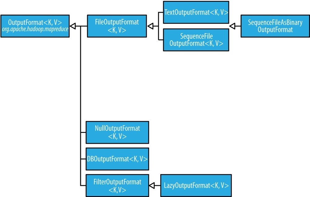
Figure 8-4. OutputFormat class hierarchy
Text Output
The default output format, TextOutputFormat, writes records as lines of text. Its keys and values may be of any type, since TextOutputFormat turns them to strings by calling toString() on them. Each key-value pair is separated by a tab character, although that may be changed using the mapreduce.output.textoutputformat.separator property.
The counterpart to TextOutputFormat for reading in this case is
KeyValueTextInputFormat, since it breaks lines into key-value pairs based on a configurable separator (see KeyValueTextInputFormat).
You can suppress the key or the value from the output (or both, making this output format equivalent to NullOutputFormat, which emits nothing) using a NullWritable type. This also causes no separator to be written, which makes the output suitable for reading in using TextInputFormat. Binary Output
SequenceFileOutputFormat
As the name indicates, SequenceFileOutputFormat writes sequence files for its output. This is a good choice of output if it forms the input to a further MapReduce job, since it is compact and is readily compressed. Compression is controlled via the static methods on SequenceFileOutputFormat, as described in Using Compression in MapReduce. For an example of how to use SequenceFileOutputFormat, see Sorting.
SequenceFileAsBinaryOutputFormat
SequenceFileAsBinaryOutputFormat — the counterpart to
SequenceFileAsBinaryInputFormat — writes keys and values in raw binary format into a sequence file container.
MapFileOutputFormat
MapFileOutputFormat writes map files as output. The keys in a MapFile must be added in order, so you need to ensure that your reducers emit keys in sorted order.
NOTE The reduce input keys are guaranteed to be sorted, but the output keys are under the control of the reduce function, and there is nothing in the general MapReduce contract that states that the reduce output keys have to be ordered in any way. The extra constraint of sorted reduce output keys is just needed for MapFileOutputFormat.
Multiple Outputs
FileOutputFormat and its subclasses generate a set of files in the output directory. There is one file per reducer, and files are named by the partition number: part-r-00000, part-r00001, and so on. Sometimes there is a need to have more control over the naming of the files or to produce multiple files per reducer. MapReduce comes with the
MultipleOutputs class to help you do this.60]
An example: Partitioning data
Consider the problem of partitioning the weather dataset by weather station. We would like to run a job whose output is one file per station, with each file containing all the records for that station.
One way of doing this is to have a reducer for each weather station. To arrange this, we need to do two things. First, write a partitioner that puts records from the same weather station into the same partition. Second, set the number of reducers on the job to be the number of weather stations. The partitioner would look like this:
public class StationPartitioner extends Partitioner
private NcdcRecordParser parser = new NcdcRecordParser();
@Override
public int getPartition(LongWritable key, Text value, int numPartitions) { parser.parse(value);
return getPartition(parser.getStationId());
}
private int getPartition(String stationId) {
…
}
}
The getPartition(String) method, whose implementation is not shown, turns the station ID into a partition index. To do this, it needs a list of all the station IDs; it then just returns the index of the station ID in the list.
There are two drawbacks to this approach. The first is that since the number of partitions needs to be known before the job is run, so does the number of weather stations. Although the NCDC provides metadata about its stations, there is no guarantee that the IDs encountered in the data will match those in the metadata. A station that appears in the metadata but not in the data wastes a reduce task. Worse, a station that appears in the data but not in the metadata doesn’t get a reduce task; it has to be thrown away. One way of mitigating this problem would be to write a job to extract the unique station IDs, but it’s a shame that we need an extra job to do this.
The second drawback is more subtle. It is generally a bad idea to allow the number of partitions to be rigidly fixed by the application, since this can lead to small or unevensized partitions. Having many reducers doing a small amount of work isn’t an efficient way of organizing a job; it’s much better to get reducers to do more work and have fewer of them, as the overhead in running a task is then reduced. Uneven-sized partitions can be difficult to avoid, too. Different weather stations will have gathered a widely varying amount of data; for example, compare a station that opened one year ago to one that has been gathering data for a century. If a few reduce tasks take significantly longer than the others, they will dominate the job execution time and cause it to be longer than it needs to be.
that the more cluster resources there are available, the faster the job can complete. This is why the default HashPartitioner works so well: it works with any number of partitions and ensures each partition has a good mix of keys, leading to more evenly sized partitions.
If we go back to using HashPartitioner, each partition will contain multiple stations, so to create a file per station, we need to arrange for each reducer to write multiple files. This is where MultipleOutputs comes in.
MultipleOutputs
MultipleOutputs allows you to write data to files whose names are derived from the output keys and values, or in fact from an arbitrary string. This allows each reducer (or mapper in a map-only job) to create more than a single file. Filenames are of the form name-m-nnnnn for map outputs and name-r-nnnnn for reduce outputs, where name is an arbitrary name that is set by the program and nnnnn is an integer designating the part number, starting from 00000. The part number ensures that outputs written from different partitions (mappers or reducers) do not collide in the case of the same name.
The program in Example 8-5 shows how to use MultipleOutputs to partition the dataset by station.
Example 8-5. Partitioning whole dataset into files named by the station ID using MultipleOutputs
public class PartitionByStationUsingMultipleOutputs extends Configured implements Tool {
static class StationMapper extends Mapper
private NcdcRecordParser parser = new NcdcRecordParser();
@Override
protected void map(LongWritable key, Text value, Context context) throws IOException, InterruptedException { parser.parse(value); context.write(new Text(parser.getStationId()), value);
}
}
static class MultipleOutputsReducer
extends Reducer
private MultipleOutputs
@Override
protected void setup(Context context) throws IOException, InterruptedException {
multipleOutputs = new MultipleOutputs
@Override
protected void reduce(Text key, Iterable
multipleOutputs.write(NullWritable.get(), value, key.toString());
}
}
@Override
protected void cleanup(Context context) throws IOException, InterruptedException { multipleOutputs.close();
}
}
@Override
public int run(String[] args) throws Exception {
Job job = JobBuilder.parseInputAndOutput(this, getConf(), args); if (job == null) { return -1;
}
job.setMapperClass(StationMapper.class); job.setMapOutputKeyClass(Text.class); job.setReducerClass(MultipleOutputsReducer.class); job.setOutputKeyClass(NullWritable.class);
return job.waitForCompletion(true) ? 0 : 1;
}
public static void main(String[] args) throws Exception { int exitCode = ToolRunner.run(new PartitionByStationUsingMultipleOutputs(), args);
System.exit(exitCode);
} }
In the reducer, which is where we generate the output, we construct an instance of MultipleOutputs in the setup() method and assign it to an instance variable. We then use the MultipleOutputs instance in the reduce() method to write to the output, in place of the context. The write() method takes the key and value, as well as a name. We use the station identifier for the name, so the overall effect is to produce output files with the naming scheme station_identifier-r-nnnnn.
In one run, the first few output files were named as follows:
output/010010-99999-r-00027 output/010050-99999-r-00013 output/010100-99999-r-00015 output/010280-99999-r-00014 output/010550-99999-r-00000 output/010980-99999-r-00011 output/011060-99999-r-00025 output/012030-99999-r-00029 output/012350-99999-r-00018 output/012620-99999-r-00004
The base path specified in the write() method of MultipleOutputs is interpreted relative to the output directory, and because it may contain file path separator characters (/), it’s possible to create subdirectories of arbitrary depth. For example, the following modification partitions the data by station and year so that each year’s data is contained in a directory named by the station ID (such as 029070-99999/1901/part-r-00000):
@Override
protected void reduce(Text key, Iterable
String basePath = String.format(“%s/%s/part”, parser.getStationId(), parser.getYear()); multipleOutputs.write(NullWritable.get(), value, basePath);
} }
MultipleOutputs delegates to the mapper’s OutputFormat. In this example it’s a TextOutputFormat, but more complex setups are possible. For example, you can create named outputs, each with its own OutputFormat and key and value types (which may differ from the output types of the mapper or reducer). Furthermore, the mapper or reducer (or both) may write to multiple output files for each record processed. Consult the Java documentation for more information.
Lazy Output
FileOutputFormat subclasses will create output (part-r-nnnnn) files, even if they are empty. Some applications prefer that empty files not be created, which is where
LazyOutputFormat helps. It is a wrapper output format that ensures that the output file is created only when the first record is emitted for a given partition. To use it, call its setOutputFormatClass() method with the JobConf and the underlying output format.
Streaming supports a -lazyOutput option to enable LazyOutputFormat.
Database Output
The output formats for writing to relational databases and to HBase are mentioned in Database Input (and Output).
[55] But see the classes in org.apache.hadoop.mapred for the old MapReduce API counterparts.
[56] This is how the mapper in SortValidator.RecordStatsChecker is implemented.
[57] In the method name isSplitable(), “splitable” has a single “t.” It is usually spelled “splittable,” which is the spelling I have used in this book.
[58] See Mahout’s XmlInputFormat for an improved XML input format.
[59] Met Office data is generally available only to the research and academic community. However, there is a small amount of monthly weather station data available at http://www.metoffice.gov.uk/climate/uk/stationdata/.
[60] The old MapReduce API includes two classes for producing multiple outputs: MultipleOutputFormat and
MultipleOutputs. In a nutshell, MultipleOutputs is more fully featured, but MultipleOutputFormat has more control over the output directory structure and file naming. MultipleOutputs in the new API combines the best features of the two multiple output classes in the old API. The code on this book’s website includes old API equivalents of the examples in this section using both MultipleOutputs and MultipleOutputFormat.
Chapter 9. MapReduce Features
This chapter looks at some of the more advanced features of MapReduce, including counters and sorting and joining datasets.
Counters
There are often things that you would like to know about the data you are analyzing but that are peripheral to the analysis you are performing. For example, if you were counting invalid records and discovered that the proportion of invalid records in the whole dataset was very high, you might be prompted to check why so many records were being marked as invalid — perhaps there is a bug in the part of the program that detects invalid records? Or if the data was of poor quality and genuinely did have very many invalid records, after discovering this, you might decide to increase the size of the dataset so that the number of good records was large enough for meaningful analysis.
Counters are a useful channel for gathering statistics about the job: for quality control or for application-level statistics. They are also useful for problem diagnosis. If you are tempted to put a log message into your map or reduce task, it is often better to see whether you can use a counter instead to record that a particular condition occurred. In addition to counter values being much easier to retrieve than log output for large distributed jobs, you get a record of the number of times that condition occurred, which is more work to obtain from a set of logfiles.
Built-in Counters
Hadoop maintains some built-in counters for every job, and these report various metrics. For example, there are counters for the number of bytes and records processed, which allow you to confirm that the expected amount of input was consumed and the expected amount of output was produced.
Counters are divided into groups, and there are several groups for the built-in counters, listed in Table 9-1.
Table 9-1. Built-in counter groups
Group Name/Enum Reference
MapReduce task counters org.apache.hadoop.mapreduce.TaskCounter Table 9-2
| Filesystem counters | org.apache.hadoop.mapreduce.FileSystemCounter | Table 9-3 |
|---|---|---|
FileInputFormat counters org.apache.hadoop.mapreduce.lib.input.FileInputFormatCounter Table 9-4<br />FileOutputFormat counters org.apache.hadoop.mapreduce.lib.output.FileOutputFormatCounter Table 9-5<br /> Job counters org.apache.hadoop.mapreduce.JobCounter Table 9-6<br /><br />Each group either contains _task counters_ (which are updated as a task progresses) or _job counters_ (which are updated as a job progresses). We look at both types in the following sections.
Task counters
Task counters gather information about tasks over the course of their execution, and the results are aggregated over all the tasks in a job. The MAPINPUT_RECORDS counter, for example, counts the input records read by each map task and aggregates over all map tasks in a job, so that the final figure is the total number of input records for the whole job.
Task counters are maintained by each task attempt, and periodically sent to the application master so they can be globally aggregated. (This is described in Progress and Status Updates.) Task counters are sent in full every time, rather than sending the counts since the last transmission, since this guards against errors due to lost messages. Furthermore, during a job run, counters may go down if a task fails.
Counter values are definitive only once a job has successfully completed. However, some counters provide useful diagnostic information as a task is progressing, and it can be useful to monitor them with the web UI. For example, PHYSICAL_MEMORY_BYTES, VIRTUAL_MEMORY_BYTES, and COMMITTED_HEAP_BYTES provide an indication of how memory usage varies over the course of a particular task attempt.
The built-in task counters include those in the MapReduce task counters group (Table 9-2) and those in the file-related counters groups (Tables 9-3, 9-4, and 9-5).
_Table 9-2. Built-in MapReduce task counters
Counter Description
| Map input records (MAP_INPUT_RECORDS) |
The number of input records consumed by all the maps in the job. Incremented every time a record is read from a RecordReader and passed to the map’s map() method by the framework. |
|---|---|
| Split raw bytes (SPLIT_RAW_BYTES) | The number of bytes of input-split objects read by maps. These objects represent the split metadata (that is, the offset and length within a file) rather than the split data itself, so the total size should be small. |
| Map output records (MAP_OUTPUT_RECORDS) |
The number of map output records produced by all the maps in the job. Incremented every time the collect() method is called on a map’s OutputCollector. |
| Map output bytes (MAP_OUTPUT_BYTES) |
The number of bytes of uncompressed output produced by all the maps in the job. Incremented every time the collect() method is called on a map’s OutputCollector. |
Map output materialized bytes The number of bytes of map output actually written to disk. If map output (MAP_OUTPUT_MATERIALIZED_BYTES) compression is enabled, this is reflected in the counter value.
| Combine input records (COMBINE_INPUT_RECORDS) |
The number of input records consumed by all the combiners (if any) in the job. Incremented every time a value is read from the combiner’s iterator over values. Note that this count is the number of values consumed by the combiner, not the number of distinct key groups (which would not be a useful metric, since there is not necessarily one group per key for a combiner; see Combiner Functions, and also Shuffle and Sort). |
||
|---|---|---|---|
| Combine output records (COMBINE_OUTPUT_RECORDS) |
The number of output records produced by all the combiners (if any) in the job. Incremented every time the collect() method is called on a combiner’s OutputCollector. | ||
| Reduce input groups (REDUCE_INPUT_GROUPS) |
The number of distinct key groups consumed by all the reducers in the job. Incremented every time the reducer’s reduce() method is called by the framework. | ||
| Reduce input records (REDUCE_INPUT_RECORDS) |
The number of input records consumed by all the reducers in the job. Incremented every time a value is read from the reducer’s iterator over values. If reducers consume all of their inputs, this count should be the same as the count for map output records. |
||
| Reduce output records (REDUCE_OUTPUT_RECORDS) |
The number of reduce output records produced by all the maps in the job. Incremented every time the collect() method is called on a reducer’s OutputCollector. | ||
| Reduce shuffle bytes (REDUCE_SHUFFLE_BYTES) |
The number of bytes of map output copied by the shuffle to reducers. | ||
| Spilled records (SPILLED_RECORDS) | The number of records spilled to disk in all map and reduce tasks in the job. | ||
| CPU milliseconds (CPU_MILLISECONDS) |
The cumulative CPU time for a task in milliseconds, as reported by /proc/cpuinfo. | ||
| Physical memory bytes (PHYSICAL_MEMORY_BYTES) |
The physical memory being used by a task in bytes, as reported by /proc/meminfo. | ||
| Virtual memory bytes (VIRTUAL_MEMORY_BYTES) |
The virtual memory being used by a task in bytes, as reported by /proc/meminfo. | ||
| Committed heap bytes (COMMITTED_HEAP_BYTES) |
The total amount of memory available in the JVM in bytes, as reported by Runtime.getRuntime().totalMemory(). | ||
| GC time milliseconds (GC_TIME_MILLIS) |
The elapsed time for garbage collection in tasks in milliseconds, as reported by GarbageCollectorMXBean.getCollectionTime(). | ||
| Shuffled maps (SHUFFLED_MAPS) | The number of map output files transferred to reducers by the shuffle (see Shuffle and Sort). | ||
| Failed shuffle (FAILED_SHUFFLE) | The number of map output copy failures during the shuffle. | ||
| Merged map outputs (MERGED_MAP_OUTPUTS) |
The number of map outputs that have been merged on the reduce side of the shuffle. | ||
| Table 9-3. Built-in filesystem task counters | |||
| Counter | Description | ||
| Filesystem bytes read (BYTES_READ) |
The number of bytes read by the filesystem by map and reduce tasks. There is a counter for each filesystem, and Filesystem may be Local, HDFS, S3, etc. | ||
| Filesystem bytes written (BYTES_WRITTEN) |
The number of bytes written by the filesystem by map and reduce tasks. | ||
| Filesystem read ops (READ_OPS) |
The number of read operations (e.g., open, file status) by the filesystem by map and reduce tasks. | ||
| Filesystem large read ops (LARGE_READ_OPS) |
The number of large read operations (e.g., list directory for a large directory) by the filesystem by map and reduce tasks. | ||
| Filesystem write ops (WRITE_OPS) |
The number of write operations (e.g., create, append) by the filesystem by map and reduce tasks. | ||
Table 9-4. Built-in FileInputFormat task counters
Counter Description Bytes read (BYTESREAD) The number of bytes read by map tasks via the FileInputFormat.
_Table 9-5. Built-in FileOutputFormat task counters
Counter Description
Bytes written The number of bytes written by map tasks (for map-only jobs) or reduce tasks via the (BYTES_WRITTEN) FileOutputFormat.
Job counters
Job counters (Table 9-6) are maintained by the application master, so they don’t need to be sent across the network, unlike all other counters, including user-defined ones. They measure job-level statistics, not values that change while a task is running. For example, TOTALLAUNCHED_MAPS counts the number of map tasks that were launched over the course of a job (including tasks that failed).
_Table 9-6. Built-in job counters
Counter Description
Launched map tasks The number of map tasks that were launched. Includes tasks that were started (TOTAL_LAUNCHED_MAPS) speculatively (see Speculative Execution).
| Launched reduce tasks (TOTAL_LAUNCHED_REDUCES) |
The number of reduce tasks that were launched. Includes tasks that were started speculatively. |
|---|---|
Launched uber tasks The number of uber tasks (see Anatomy of a MapReduce Job Run) that were launched. (TOTAL_LAUNCHED_UBERTASKS)
| Maps in uber tasks (NUM_UBER_SUBMAPS) |
The number of maps in uber tasks. |
|---|---|
| Reduces in uber tasks (NUM_UBER_SUBREDUCES) |
The number of reduces in uber tasks. |
| Failed map tasks (NUM_FAILED_MAPS) |
The number of map tasks that failed. See Task Failure for potential causes. |
| Failed reduce tasks (NUM_FAILED_REDUCES) |
The number of reduce tasks that failed. |
| Failed uber tasks (NUM_FAILED_UBERTASKS) |
The number of uber tasks that failed. |
| Killed map tasks (NUM_KILLED_MAPS) |
The number of map tasks that were killed. See Task Failure for potential causes. |
| Killed reduce tasks (NUM_KILLED_REDUCES) |
The number of reduce tasks that were killed. |
| Data-local map tasks (DATA_LOCAL_MAPS) |
The number of map tasks that ran on the same node as their input data. |
| Rack-local map tasks (RACK_LOCAL_MAPS) |
The number of map tasks that ran on a node in the same rack as their input data, but were not data-local. |
| Other local map tasks (OTHER_LOCAL_MAPS) |
The number of map tasks that ran on a node in a different rack to their input data. Interrack bandwidth is scarce, and Hadoop tries to place map tasks close to their input data, so this count should be low. See Figure 2-2. |
| Total time in map tasks (MILLIS_MAPS) |
The total time taken running map tasks, in milliseconds. Includes tasks that were started speculatively. See also corresponding counters for measuring core and memory usage (VCORES_MILLIS_MAPS and MB_MILLIS_MAPS). |
| Total time in reduce tasks (MILLIS_REDUCES) |
The total time taken running reduce tasks, in milliseconds. Includes tasks that were started speculatively. See also corresponding counters for measuring core and memory usage (VCORES_MILLIS_REDUCES and MB_MILLIS_REDUCES). |
User-Defined Java Counters
MapReduce allows user code to define a set of counters, which are then incremented as desired in the mapper or reducer. Counters are defined by a Java enum, which serves to group related counters. A job may define an arbitrary number of enums, each with an arbitrary number of fields. The name of the enum is the group name, and the enum’s fields are the counter names. Counters are global: the MapReduce framework aggregates them across all maps and reduces to produce a grand total at the end of the job.
We created some counters in Chapter 6 for counting malformed records in the weather dataset. The program in Example 9-1 extends that example to count the number of missing records and the distribution of temperature quality codes.
Example 9-1. Application to run the maximum temperature job, including counting missing and malformed fields and quality codes
public class MaxTemperatureWithCounters extends Configured implements Tool {
enum Temperature {
MISSING,
MALFORMED
}
static class MaxTemperatureMapperWithCounters extends Mapper
private NcdcRecordParser parser = new NcdcRecordParser();
@Override
protected void map(LongWritable key, Text value, Context context) throws IOException, InterruptedException {
parser.parse(value); if (parser.isValidTemperature()) { int airTemperature = parser.getAirTemperature(); context.write(new Text(parser.getYear()), new IntWritable(airTemperature));
} else if (parser.isMalformedTemperature()) {
System.err.println(“Ignoring possibly corrupt input: “ + value); context.getCounter(Temperature.MALFORMED).increment(1);
} else if (parser.isMissingTemperature()) {
context.getCounter(Temperature.MISSING).increment(1);
}
// dynamic counter
context.getCounter(“TemperatureQuality”, parser.getQuality()).increment(1);
}
}
@Override
public int run(String[] args) throws Exception {
Job job = JobBuilder.parseInputAndOutput(this, getConf(), args); if (job == null) { return -1;
}
job.setOutputKeyClass(Text.class); job.setOutputValueClass(IntWritable.class);
job.setMapperClass(MaxTemperatureMapperWithCounters.class); job.setCombinerClass(MaxTemperatureReducer.class); job.setReducerClass(MaxTemperatureReducer.class);
return job.waitForCompletion(true) ? 0 : 1;
}
public static void main(String[] args) throws Exception { int exitCode = ToolRunner.run(new MaxTemperatureWithCounters(), args);
System.exit(exitCode);
} }
The best way to see what this program does is to run it over the complete dataset:
% hadoop jar hadoop-examples.jar MaxTemperatureWithCounters \ input/ncdc/all output-counters
When the job has successfully completed, it prints out the counters at the end (this is done by the job client). Here are the ones we are interested in:
Air Temperature Records
Malformed=3
Missing=66136856 TemperatureQuality
0=1
1=973422173 2=1246032 4=10764500
5=158291879
6=40066
9=66136858
Notice that the counters for temperature have been made more readable by using a resource bundle named after the enum (using an underscore as a separator for nested classes) — in this case MaxTemperatureWithCounters_Temperature.properties, which contains the display name mappings.
Dynamic counters
The code makes use of a dynamic counter — one that isn’t defined by a Java enum. Because a Java enum’s fields are defined at compile time, you can’t create new counters on the fly using enums. Here we want to count the distribution of temperature quality codes, and though the format specification defines the values that the temperature quality code can take, it is more convenient to use a dynamic counter to emit the values that it actually takes. The method we use on the Context object takes a group and counter name using String names:
public Counter getCounter(String groupName, String counterName)
The two ways of creating and accessing counters — using enums and using strings — are actually equivalent because Hadoop turns enums into strings to send counters over RPC.
Enums are slightly easier to work with, provide type safety, and are suitable for most jobs. For the odd occasion when you need to create counters dynamically, you can use the String interface.
Retrieving counters
In addition to using the web UI and the command line (using mapred job -counter), you can retrieve counter values using the Java API. You can do this while the job is running, although it is more usual to get counters at the end of a job run, when they are stable. Example 9-2 shows a program that calculates the proportion of records that have missing temperature fields.
Example 9-2. Application to calculate the proportion of records with missing temperature fields
import org.apache.hadoop.conf.Configured; import org.apache.hadoop.mapreduce.*; import org.apache.hadoop.util.*; public class MissingTemperatureFields extends Configured implements Tool {
@Override
public int run(String[] args) throws Exception { if (args.length != 1) {
JobBuilder.printUsage(this, “
}
String jobID = args[0];
Cluster cluster = new Cluster(getConf()); Job job = cluster.getJob(JobID.forName(jobID)); if (job == null) {
System.err.printf(“No job with ID %s found.\n”, jobID); return -1;
}
if (!job.isComplete()) {
System.err.printf(“Job %s is not complete.\n”, jobID); return -1; }
Counters counters = job.getCounters(); long missing = counters.findCounter(
MaxTemperatureWithCounters.Temperature.MISSING).getValue(); long total = counters.findCounter(TaskCounter.MAP_INPUT_RECORDS).getValue();
System.out.printf(“Records with missing temperature fields: %.2f%%\n”,
100.0 missing / total); return 0;
}
public static void main(String[] args) throws Exception { int exitCode = ToolRunner.run(new MissingTemperatureFields(), args);
System.exit(exitCode);
} }
First we retrieve a Job object from a Cluster by calling the getJob() method with the job ID. We check whether there is actually a job with the given ID by checking if it is null. There may not be, either because the ID was incorrectly specified or because the job is no longer in the job history.
After confirming that the job has completed, we call the Job’s getCounters() method, which returns a Counters object encapsulating all the counters for the job. The Counters class provides various methods for finding the names and values of counters. We use the findCounter() method, which takes an enum to find the number of records that had a missing temperature field and also the total number of records processed (from a built-in counter).
Finally, we print the proportion of records that had a missing temperature field. Here’s what we get for the whole weather dataset:
% *hadoop jar hadoop-examples.jar MissingTemperatureFields job_1410450250506_0007 Records with missing temperature fields: 5.47%
User-Defined Streaming Counters
A Streaming MapReduce program can increment counters by sending a specially formatted line to the standard error stream, which is co-opted as a control channel in this case. The line must have the following format: reporter:counter:group,counter,amount
This snippet in Python shows how to increment the “Missing” counter in the “Temperature” group by 1: sys.stderr.write(“reporter:counter:Temperature,Missing,1\n“)
In a similar way, a status message may be sent with a line formatted like this:
reporter:status:message
Sorting
The ability to sort data is at the heart of MapReduce. Even if your application isn’t concerned with sorting per se, it may be able to use the sorting stage that MapReduce provides to organize its data. In this section, we examine different ways of sorting datasets and how you can control the sort order in MapReduce. Sorting Avro data is covered separately, in Sorting Using Avro MapReduce.
Preparation
We are going to sort the weather dataset by temperature. Storing temperatures as Text objects doesn’t work for sorting purposes, because signed integers don’t sort lexicographically.61] Instead, we are going to store the data using sequence files whose IntWritable keys represent the temperatures (and sort correctly) and whose Text values are the lines of data.
The MapReduce job in Example 9-3 is a map-only job that also filters the input to remove records that don’t have a valid temperature reading. Each map creates a single blockcompressed sequence file as output. It is invoked with the following command:
% hadoop jar hadoop-examples.jar SortDataPreprocessor input/ncdc/all \ input/ncdc/all-seq
Example 9-3. A MapReduce program for transforming the weather data into SequenceFile format
public class SortDataPreprocessor extends Configured implements Tool {
static class CleanerMapper extends Mapper
private NcdcRecordParser parser = new NcdcRecordParser();
@Override
protected void map(LongWritable key, Text value, Context context) throws IOException, InterruptedException {
parser.parse(value); if (parser.isValidTemperature()) { context.write(new IntWritable(parser.getAirTemperature()), value);
}
}
}
@Override
public int run(String[] args) throws Exception {
Job job = JobBuilder.parseInputAndOutput(this, getConf(), args); if (job == null) { return -1;
}
job.setMapperClass(CleanerMapper.class); job.setOutputKeyClass(IntWritable.class); job.setOutputValueClass(Text.class); job.setNumReduceTasks(0); job.setOutputFormatClass(SequenceFileOutputFormat.class);
SequenceFileOutputFormat.setCompressOutput(job, true);
SequenceFileOutputFormat.setOutputCompressorClass(job, GzipCodec.class);
SequenceFileOutputFormat.setOutputCompressionType(job, CompressionType.BLOCK);
return job.waitForCompletion(true) ? 0 : 1;
}
public static void main(String[] args) throws Exception {
int exitCode = ToolRunner.run(new SortDataPreprocessor(), args); System.exit(exitCode);
} }
Partial Sort
In The Default MapReduce Job, we saw that, by default, MapReduce will sort input records by their keys. Example 9-4 is a variation for sorting sequence files with IntWritable keys.
Example 9-4. A MapReduce program for sorting a SequenceFile with IntWritable keys using the default HashPartitioner
public class SortByTemperatureUsingHashPartitioner extends Configured implements Tool {
@Override
public int run(String[] args) throws Exception {
Job job = JobBuilder.parseInputAndOutput(this, getConf(), args); if (job == null) { return -1;
}
job.setInputFormatClass(SequenceFileInputFormat.class); job.setOutputKeyClass(IntWritable.class); job.setOutputFormatClass(SequenceFileOutputFormat.class);
SequenceFileOutputFormat.setCompressOutput(job, true);
SequenceFileOutputFormat.setOutputCompressorClass(job, GzipCodec.class);
SequenceFileOutputFormat.setOutputCompressionType(job,
CompressionType.BLOCK);
return job.waitForCompletion(true) ? 0 : 1;
}
public static void main(String[] args) throws Exception { int exitCode = ToolRunner.run(new SortByTemperatureUsingHashPartitioner(), args);
System.exit(exitCode);
}
}
CONTROLLING SORT ORDER
The sort order for keys is controlled by a RawComparator, which is found as follows:
1. If the property mapreduce.job.output.key.comparator.class is set, either explicitly or by calling setSortComparatorClass() on Job, then an instance of that class is used. (In the old API, the equivalent method is setOutputKeyComparatorClass() on JobConf.)
2. Otherwise, keys must be a subclass of WritableComparable, and the registered comparator for the key class is used.
3. If there is no registered comparator, then a RawComparator is used. The RawComparator deserializes the byte streams being compared into objects and delegates to the WritableComparable’s compareTo() method. These rules reinforce the importance of registering optimized versions of RawComparators for your own custom Writable classes (which is covered in Implementing a RawComparator for speed), and also show that it’s straightforward to override the sort order by setting your own comparator (we do this in Secondary Sort).
Suppose we run this program using 30 reducers:62]
% hadoop jar hadoop-examples.jar SortByTemperatureUsingHashPartitioner \
-D mapreduce.job.reduces=30 input/ncdc/all-seq output-hashsort
This command produces 30 output files, each of which is sorted. However, there is no easy way to combine the files (by concatenation, for example, in the case of plain-text files) to produce a globally sorted file.
For many applications, this doesn’t matter. For example, having a partially sorted set of files is fine when you want to do lookups by key. The SortByTemperatureToMapFile and LookupRecordsByTemperature classes in this book’s example code explore this idea. By using a map file instead of a sequence file, it’s possible to first find the relevant partition that a key belongs in (using the partitioner), then to do an efficient lookup of the record within the map file partition.
Total Sort
How can you produce a globally sorted file using Hadoop? The naive answer is to use a single partition.63] But this is incredibly inefficient for large files, because one machine has to process all of the output, so you are throwing away the benefits of the parallel architecture that MapReduce provides.
Instead, it is possible to produce a set of sorted files that, if concatenated, would form a globally sorted file. The secret to doing this is to use a partitioner that respects the total order of the output. For example, if we had four partitions, we could put keys for temperatures less than –10°C in the first partition, those between –10°C and 0°C in the second, those between 0°C and 10°C in the third, and those over 10°C in the fourth.
Although this approach works, you have to choose your partition sizes carefully to ensure that they are fairly even, so job times aren’t dominated by a single reducer. For the partitioning scheme just described, the relative sizes of the partitions are as follows:
| Temperature range | < –10°C | [–10°C, 0°C) | [0°C, 10°C) | >= 10°C |
|---|---|---|---|---|
| Proportion of records | 11% | 13% | 17% | 59% |
These partitions are not very even. To construct more even partitions, we need to have a better understanding of the temperature distribution for the whole dataset. It’s fairly easy to write a MapReduce job to count the number of records that fall into a collection of temperature buckets. For example, Figure 9-1 shows the distribution for buckets of size 1°C, where each point on the plot corresponds to one bucket.
Although we could use this information to construct a very even set of partitions, the fact that we needed to run a job that used the entire dataset to construct them is not ideal. It’s possible to get a fairly even set of partitions by sampling the key space. The idea behind sampling is that you look at a small subset of the keys to approximate the key distribution, which is then used to construct partitions. Luckily, we don’t have to write the code to do this ourselves, as Hadoop comes with a selection of samplers.
The InputSampler class defines a nested Sampler interface whose implementations return a sample of keys given an InputFormat and Job:
public interface Sampler
K[] getSample(InputFormat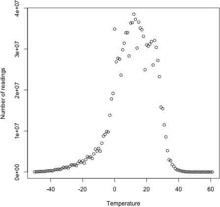
Figure 9-1. Temperature distribution for the weather dataset
This interface usually is not called directly by clients. Instead, the writePartitionFile() static method on InputSampler is used, which creates a sequence file to store the keys that define the partitions:
public static
The sequence file is used by TotalOrderPartitioner to create partitions for the sort job. Example 9-5 puts it all together.
Example 9-5. A MapReduce program for sorting a SequenceFile with IntWritable keys using the TotalOrderPartitioner to globally sort the data
public class SortByTemperatureUsingTotalOrderPartitioner extends Configured implements Tool {
@Override
public int run(String[] args) throws Exception {
Job job = JobBuilder.parseInputAndOutput(this, getConf(), args); if (job == null) { return -1;
}
job.setInputFormatClass(SequenceFileInputFormat.class); job.setOutputKeyClass(IntWritable.class); job.setOutputFormatClass(SequenceFileOutputFormat.class);
SequenceFileOutputFormat.setCompressOutput(job, true);
SequenceFileOutputFormat.setOutputCompressorClass(job, GzipCodec.class);
SequenceFileOutputFormat.setOutputCompressionType(job, CompressionType.BLOCK); job.setPartitionerClass(TotalOrderPartitioner.class);
InputSampler.Sampler
new InputSampler.RandomSampler
InputSampler.writePartitionFile(job, sampler);
// Add to DistributedCache
Configuration conf = job.getConfiguration();
String partitionFile = TotalOrderPartitioner.getPartitionFile(conf);
URI partitionUri = new URI(partitionFile); job.addCacheFile(partitionUri);
return job.waitForCompletion(true) ? 0 : 1;
}
public static void main(String[] args) throws Exception { int exitCode = ToolRunner.run( new SortByTemperatureUsingTotalOrderPartitioner(), args);
System.exit(exitCode);
} }
We use a RandomSampler, which chooses keys with a uniform probability — here, 0.1. There are also parameters for the maximum number of samples to take and the maximum number of splits to sample (here, 10,000 and 10, respectively; these settings are the defaults when InputSampler is run as an application), and the sampler stops when the first of these limits is met. Samplers run on the client, making it important to limit the number of splits that are downloaded so the sampler runs quickly. In practice, the time taken to run the sampler is a small fraction of the overall job time.
The InputSampler writes a partition file that we need to share with the tasks running on the cluster by adding it to the distributed cache (see Distributed Cache).
On one run, the sampler chose –5.6°C, 13.9°C, and 22.0°C as partition boundaries (for four partitions), which translates into more even partition sizes than the earlier choice:
| Temperature range | < –5.6°C | [–5.6°C, 13.9°C) | [13.9°C, 22.0°C) | >= 22.0°C |
|---|---|---|---|---|
| Proportion of records | 29% | 24% | 23% | 24% |
Your input data determines the best sampler to use. For example, SplitSampler, which samples only the first n records in a split, is not so good for sorted data,64] because it doesn’t select keys from throughout the split.
On the other hand, IntervalSampler chooses keys at regular intervals through the split and makes a better choice for sorted data. RandomSampler is a good general-purpose sampler. If none of these suits your application (and remember that the point of sampling is to produce partitions that are approximately equal in size), you can write your own implementation of the Sampler interface.
One of the nice properties of InputSampler and TotalOrderPartitioner is that you are free to choose the number of partitions — that is, the number of reducers. However, TotalOrderPartitioner will work only if the partition boundaries are distinct. One problem with choosing a high number is that you may get collisions if you have a small key space.
Here’s how we run it:
% hadoop jar hadoop-examples.jar SortByTemperatureUsingTotalOrderPartitioner \
-D mapreduce.job.reduces=30 input/ncdc/all-seq output-totalsort
The program produces 30 output partitions, each of which is internally sorted; in addition, for these partitions, all the keys in partition i are less than the keys in partition i + 1.
Secondary Sort
The MapReduce framework sorts the records by key before they reach the reducers. For any particular key, however, the values are not sorted. The order in which the values appear is not even stable from one run to the next, because they come from different map tasks, which may finish at different times from run to run. Generally speaking, most MapReduce programs are written so as not to depend on the order in which the values appear to the reduce function. However, it is possible to impose an order on the values by sorting and grouping the keys in a particular way.
To illustrate the idea, consider the MapReduce program for calculating the maximum temperature for each year. If we arranged for the values (temperatures) to be sorted in descending order, we wouldn’t have to iterate through them to find the maximum; instead, we could take the first for each year and ignore the rest. (This approach isn’t the most efficient way to solve this particular problem, but it illustrates how secondary sort works in general.)
To achieve this, we change our keys to be composite: a combination of year and temperature. We want the sort order for keys to be by year (ascending) and then by temperature (descending):
1900 35°C
1900 34°C
1900 34°C…
1901 36°C
1901 35°C
If all we did was change the key, this wouldn’t help, because then records for the same year would have different keys and therefore would not (in general) go to the same reducer. For example, (1900, 35°C) and (1900, 34°C) could go to different reducers. By setting a partitioner to partition by the year part of the key, we can guarantee that records for the same year go to the same reducer. This still isn’t enough to achieve our goal, however. A partitioner ensures only that one reducer receives all the records for a year; it doesn’t change the fact that the reducer groups by key within the partition: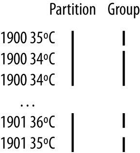
The final piece of the puzzle is the setting to control the grouping. If we group values in the reducer by the year part of the key, we will see all the records for the same year in one reduce group. And because they are sorted by temperature in descending order, the first is the maximum temperature: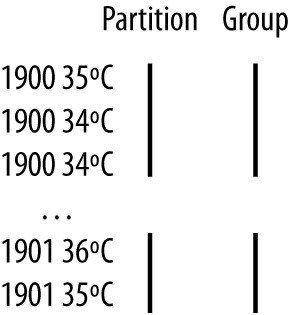
To summarize, there is a recipe here to get the effect of sorting by value: Make the key a composite of the natural key and the natural value.
The sort comparator should order by the composite key (i.e., the natural key and natural value).
The partitioner and grouping comparator for the composite key should consider only the natural key for partitioning and grouping.
Java code
Putting this all together results in the code in Example 9-6. This program uses the plaintext input again.
Example 9-6. Application to find the maximum temperature by sorting temperatures in the key
public class MaxTemperatureUsingSecondarySort extends Configured implements Tool {
static class MaxTemperatureMapper extends Mapper
private NcdcRecordParser parser = new NcdcRecordParser();
@Override
protected void map(LongWritable key, Text value,
Context context) throws IOException, InterruptedException {
parser.parse(value); if (parser.isValidTemperature()) {
context.write(new IntPair(parser.getYearInt(), parser.getAirTemperature()), NullWritable.get()); }
}
}
static class MaxTemperatureReducer extends Reducer
@Override
protected void reduce(IntPair key, Iterable
Context context) throws IOException, InterruptedException {
context.write(key, NullWritable.get()); }
} public static class FirstPartitioner extends Partitioner
@Override
public int getPartition(IntPair key, NullWritable value, int numPartitions) {
// multiply by 127 to perform some mixing
return Math.abs(key.getFirst() 127) % numPartitions;
}
}
public static class KeyComparator extends WritableComparator { protected KeyComparator() { super(IntPair.class, true);
} @Override
public int compare(WritableComparable w1, WritableComparable w2) {
IntPair ip1 = (IntPair) w1; IntPair ip2 = (IntPair) w2;
int cmp = IntPair.compare(ip1.getFirst(), ip2.getFirst()); if (cmp != 0) { return cmp;
}
return -IntPair.compare(ip1.getSecond(), ip2.getSecond()); //reverse
}
}
public static class GroupComparator extends WritableComparator { protected GroupComparator() { super(IntPair.class, true);
} @Override
public int compare(WritableComparable w1, WritableComparable w2) {
IntPair ip1 = (IntPair) w1; IntPair ip2 = (IntPair) w2;
return IntPair.compare(ip1.getFirst(), ip2.getFirst());
}
}
@Override
public int run(String[] args) throws Exception {
Job job = JobBuilder.parseInputAndOutput(this, getConf(), args); if (job == null) { return -1;
}
job.setMapperClass(MaxTemperatureMapper.class); job.setPartitionerClass(FirstPartitioner.class); job.setSortComparatorClass(KeyComparator.class); job.setGroupingComparatorClass(GroupComparator.class); job.setReducerClass(MaxTemperatureReducer.class); job.setOutputKeyClass(IntPair.class); job.setOutputValueClass(NullWritable.class);
return job.waitForCompletion(true) ? 0 : 1; }
public static void main(String[] args) throws Exception { int exitCode = ToolRunner.run(new MaxTemperatureUsingSecondarySort(), args);
System.exit(exitCode);
} }
In the mapper, we create a key representing the year and temperature, using an IntPair
Writable implementation. (IntPair is like the TextPair class we developed in Implementing a Custom Writable.) We don’t need to carry any information in the value, because we can get the first (maximum) temperature in the reducer from the key, so we use a NullWritable. The reducer emits the first key, which, due to the secondary sorting, is an IntPair for the year and its maximum temperature. IntPair’s toString() method creates a tab-separated string, so the output is a set of tab-separated year-temperature pairs.
NOTE Many applications need to access all the sorted values, not just the first value as we have provided here. To do this, you need to populate the value fields since in the reducer you can retrieve only the first key. This necessitates some unavoidable duplication of information between key and value.
We set the partitioner to partition by the first field of the key (the year) using a custom partitioner called FirstPartitioner. To sort keys by year (ascending) and temperature (descending), we use a custom sort comparator, using setSortComparatorClass(), that extracts the fields and performs the appropriate comparisons. Similarly, to group keys by year, we set a custom comparator, using setGroupingComparatorClass(), to extract the first field of the key for comparison.65]
Running this program gives the maximum temperatures for each year:
% hadoop jar hadoop-examples.jar MaxTemperatureUsingSecondarySort \ input/ncdc/all output-secondarysort
% **hadoop fs -cat output-secondarysort/part- | sort | head**
1901 317
1902 244
1903 289
1904 256
1905 283
1906 294
1907 283
1908 289
1909 278
1910 294
Streaming
To do a secondary sort in Streaming, we can take advantage of a couple of library classes that Hadoop provides. Here’s the driver that we can use to do a secondary sort:
% hadoop jar $HADOOP_HOME/share/hadoop/tools/lib/hadoop-streaming-*.jar \
-D stream.num.map.output.key.fields=2 \
-D mapreduce.partition.keypartitioner.options=-k1,1 \ -D mapreduce.job.output.key.comparator.class=\ org.apache.hadoop.mapred.lib.KeyFieldBasedComparator \
-D mapreduce.partition.keycomparator.options=”-k1n -k2nr” \ -files secondary_sort_map.py,secondary_sort_reduce.py \
-input input/ncdc/all \
-output output-secondarysort-streaming \
-mapper ch09-mr-features/src/main/python/secondary_sort_map.py \
-partitioner org.apache.hadoop.mapred.lib.KeyFieldBasedPartitioner \
-reducer ch09-mr-features/src/main/python/secondary_sort_reduce.py
Our map function (Example 9-7) emits records with year and temperature fields. We want to treat the combination of both of these fields as the key, so we set stream.num.map.output.key.fields to 2. This means that values will be empty, just like in the Java case.
Example 9-7. Map function for secondary sort in Python
#!/usr/bin/env python
import re import sys
for line in sys.stdin: val = line.strip()
(year, temp, q) = (val[15:19], int(val[87:92]), val[92:93]) if temp == 9999:
sys.stderr.write(“reporter:counter:Temperature,Missing,1\n“) elif re.match(“[01459]”, q): print “%s\t%s” % (year, temp)
However, we don’t want to partition by the entire key, so we use
KeyFieldBasedPartitioner, which allows us to partition by a part of the key. The specification mapreduce.partition.keypartitioner.options configures the partitioner. The value -k1,1 instructs the partitioner to use only the first field of the key, where fields are assumed to be separated by a string defined by the mapreduce.map.output.key.field.separator property (a tab character by default).
Next, we want a comparator that sorts the year field in ascending order and the temperature field in descending order, so that the reduce function can simply return the first record in each group. Hadoop provides KeyFieldBasedComparator, which is ideal for this purpose. The comparison order is defined by a specification that is like the one used for GNU sort. It is set using the mapreduce.partition.keycomparator.options property. The value -k1n -k2nr used in this example means “sort by the first field in numerical order, then by the second field in reverse numerical order.” Like its partitioner cousin, KeyFieldBasedPartitioner, it uses the map output key separator to split a key into fields.
In the Java version, we had to set the grouping comparator; however, in Streaming, groups are not demarcated in any way, so in the reduce function we have to detect the group boundaries ourselves by looking for when the year changes (Example 9-8).
Example 9-8. Reduce function for secondary sort in Python
#!/usr/bin/env python import sys
last_group = None for line in sys.stdin: val = line.strip()
(year, temp) = val.split(“\t“) group = year if last_group != group: print val last_group = group
When we run the Streaming program, we get the same output as the Java version.
Finally, note that KeyFieldBasedPartitioner and KeyFieldBasedComparator are not confined to use in Streaming programs; they are applicable to Java MapReduce programs, too.
Joins
MapReduce can perform joins between large datasets, but writing the code to do joins from scratch is fairly involved. Rather than writing MapReduce programs, you might consider using a higher-level framework such as Pig, Hive, Cascading, Cruc, or Spark, in which join operations are a core part of the implementation.
Let’s briefly consider the problem we are trying to solve. We have two datasets — for example, the weather stations database and the weather records — and we want to reconcile the two. Let’s say we want to see each station’s history, with the station’s metadata inlined in each output row. This is illustrated in Figure 9-2.
How we implement the join depends on how large the datasets are and how they are partitioned. If one dataset is large (the weather records) but the other one is small enough to be distributed to each node in the cluster (as the station metadata is), the join can be effected by a MapReduce job that brings the records for each station together (a partial sort on station ID, for example). The mapper or reducer uses the smaller dataset to look up the station metadata for a station ID, so it can be written out with each record. See Side Data Distribution for a discussion of this approach, where we focus on the mechanics of distributing the data to nodes in the cluster.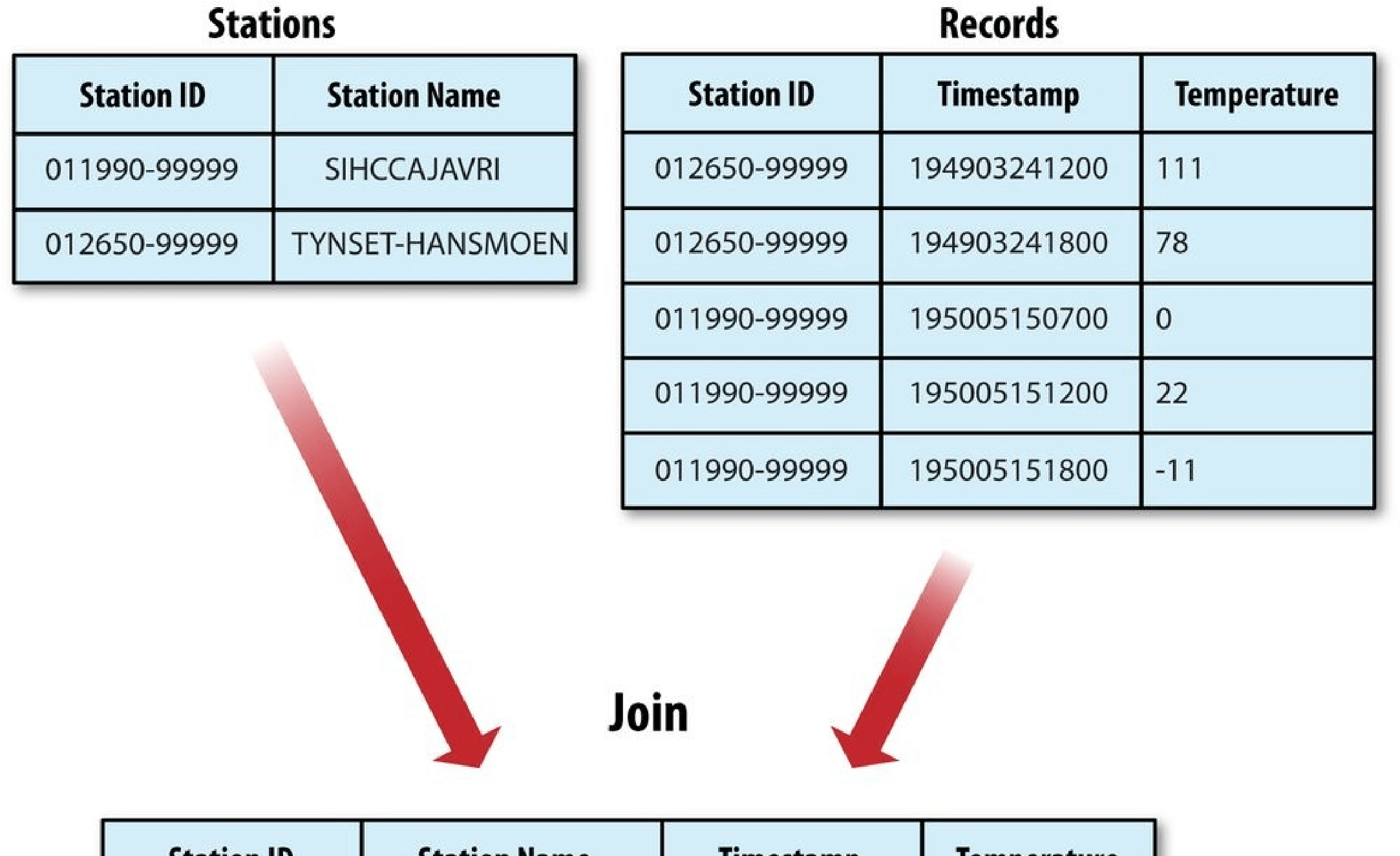
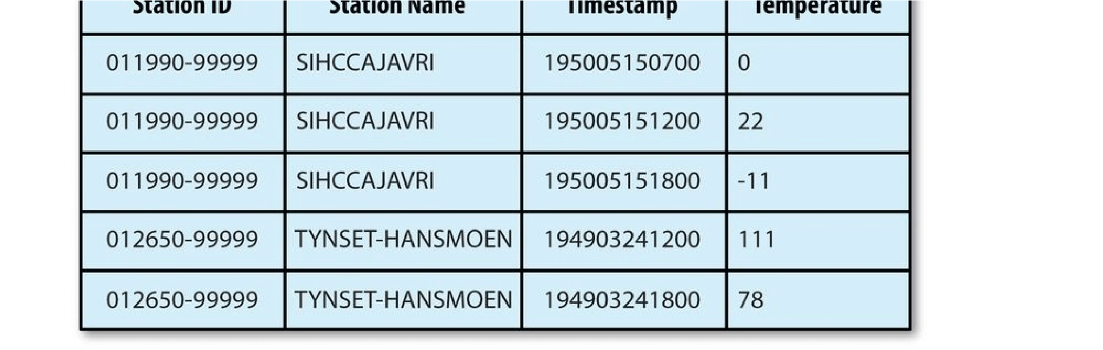
Figure 9-2. Inner join of two datasets
If the join is performed by the mapper it is called a map-side join, whereas if it is performed by the reducer it is called a reduce-side join.
If both datasets are too large for either to be copied to each node in the cluster, we can still join them using MapReduce with a map-side or reduce-side join, depending on how the data is structured. One common example of this case is a user database and a log of some user activity (such as access logs). For a popular service, it is not feasible to distribute the user database (or the logs) to all the MapReduce nodes.
Map-Side Joins
A map-side join between large inputs works by performing the join before the data reaches the map function. For this to work, though, the inputs to each map must be partitioned and sorted in a particular way. Each input dataset must be divided into the same number of partitions, and it must be sorted by the same key (the join key) in each source. All the records for a particular key must reside in the same partition. This may sound like a strict requirement (and it is), but it actually fits the description of the output of a MapReduce job.
A map-side join can be used to join the outputs of several jobs that had the same number of reducers, the same keys, and output files that are not splittable (by virtue of being smaller than an HDFS block or being gzip compressed, for example). In the context of the weather example, if we ran a partial sort on the stations file by station ID, and another identical sort on the records, again by station ID and with the same number of reducers, then the two outputs would satisfy the conditions for running a map-side join.
You use a CompositeInputFormat from the org.apache.hadoop.mapreduce.join package to run a map-side join. The input sources and join type (inner or outer) for
CompositeInputFormat are configured through a join expression that is written according to a simple grammar. The package documentation has details and examples.
The org.apache.hadoop.examples.Join example is a general-purpose command-line program for running a map-side join, since it allows you to run a MapReduce job for any specified mapper and reducer over multiple inputs that are joined with a given join operation.
Reduce-Side Joins
A reduce-side join is more general than a map-side join, in that the input datasets don’t have to be structured in any particular way, but it is less efficient because both datasets have to go through the MapReduce shuffle. The basic idea is that the mapper tags each record with its source and uses the join key as the map output key, so that the records with the same key are brought together in the reducer. We use several ingredients to make this work in practice:
Multiple inputs
The input sources for the datasets generally have different formats, so it is very convenient to use the MultipleInputs class (see Multiple Inputs) to separate the logic for parsing and tagging each source.
Secondary sort
As described, the reducer will see the records from both sources that have the same key, but they are not guaranteed to be in any particular order. However, to perform the join, it is important to have the data from one source before that from the other. For the weather data join, the station record must be the first of the values seen for each key, so the reducer can fill in the weather records with the station name and emit them straightaway. Of course, it would be possible to receive the records in any order if we buffered them in memory, but this should be avoided because the number of records in any group may be very large and exceed the amount of memory available to the reducer.
We saw in Secondary Sort how to impose an order on the values for each key that the reducers see, so we use this technique here.
To tag each record, we use TextPair (discussed in Chapter 5) for the keys (to store the station ID) and the tag. The only requirement for the tag values is that they sort in such a way that the station records come before the weather records. This can be achieved by tagging station records as 0 and weather records as 1. The mapper classes to do this are shown in Examples 9-9 and 9-10.
Example 9-9. Mapper for tagging station records for a reduce-side join
public class JoinStationMapper
extends Mapper
private NcdcStationMetadataParser parser = new NcdcStationMetadataParser();
@Override
protected void map(LongWritable key, Text value, Context context) throws IOException, InterruptedException { if (parser.parse(value)) { context.write(new TextPair(parser.getStationId(), “0”), new Text(parser.getStationName())); }
} }
Example 9-10. Mapper for tagging weather records for a reduce-side join
public class JoinRecordMapper
extends Mapper
@Override
protected void map(LongWritable key, Text value, Context context) throws IOException, InterruptedException { parser.parse(value); context.write(new TextPair(parser.getStationId(), “1”), value);
}
}
The reducer knows that it will receive the station record first, so it extracts its name from the value and writes it out as a part of every output record (Example 9-11).
Example 9-11. Reducer for joining tagged station records with tagged weather records
public class JoinReducer extends Reducer
@Override
protected void reduce(TextPair key, Iterable
Text stationName = new Text(iter.next()); while (iter.hasNext()) {
Text record = iter.next();
Text outValue = new Text(stationName.toString() + “\t” + record.toString()); context.write(key.getFirst(), outValue);
}
} }
The code assumes that every station ID in the weather records has exactly one matching record in the station dataset. If this were not the case, we would need to generalize the code to put the tag into the value objects, by using another TextPair. The reduce() method would then be able to tell which entries were station names and detect (and
is that we partition and group on the first part of the key, the station ID, which we do with a custom Partitioner (KeyPartitioner) and a custom group comparator, FirstComparator (from TextPair).
Example 9-12. Application to join weather records with station names
public class JoinRecordWithStationName extends Configured implements Tool {
public static class KeyPartitioner extends Partitioner
@Override
public int getPartition(TextPair key, Text value, int numPartitions) { return (key.getFirst().hashCode() & Integer.MAX_VALUE) % numPartitions;
}
}
@Override
public int run(String[] args) throws Exception {
if (args.length != 3) {
JobBuilder.printUsage(this, “
Side Data Distribution
Side data can be defined as extra read-only data needed by a job to process the main dataset. The challenge is to make side data available to all the map or reduce tasks (which are spread across the cluster) in a convenient and efficient fashion.
Using the Job Configuration
You can set arbitrary key-value pairs in the job configuration using the various setter methods on Configuration (or JobConf in the old MapReduce API). This is very useful when you need to pass a small piece of metadata to your tasks.
In the task, you can retrieve the data from the configuration returned by Context’s getConfiguration() method. (In the old API, it’s a little more involved: override the configure() method in the Mapper or Reducer and use a getter method on the JobConf object passed in to retrieve the data. It’s very common to store the data in an instance field so it can be used in the map() or reduce() method.)
Usually a primitive type is sufficient to encode your metadata, but for arbitrary objects you can either handle the serialization yourself (if you have an existing mechanism for turning objects to strings and back) or use Hadoop’s Stringifier class. The
DefaultStringifier uses Hadoop’s serialization framework to serialize objects (see Serialization).
You shouldn’t use this mechanism for transferring more than a few kilobytes of data, because it can put pressure on the memory usage in MapReduce components. The job configuration is always read by the client, the application master, and the task JVM, and each time the configuration is read, all of its entries are read into memory, even if they are not used.
Distributed Cache
Rather than serializing side data in the job configuration, it is preferable to distribute datasets using Hadoop’s distributed cache mechanism. This provides a service for copying files and archives to the task nodes in time for the tasks to use them when they run. To save network bandwidth, files are normally copied to any particular node once per job.
Usage
For tools that use GenericOptionsParser (this includes many of the programs in this book; see GenericOptionsParser, Tool, and ToolRunner), you can specify the files to be distributed as a comma-separated list of URIs as the argument to the -files option. Files can be on the local filesystem, on HDFS, or on another Hadoop-readable filesystem (such as S3). If no scheme is supplied, then the files are assumed to be local. (This is true even when the default filesystem is not the local filesystem.)
You can also copy archive files (JAR files, ZIP files, tar files, and gzipped tar files) to your tasks using the -archives option; these are unarchived on the task node. The -libjars option will add JAR files to the classpath of the mapper and reducer tasks. This is useful if you haven’t bundled library JAR files in your job JAR file.
Let’s see how to use the distributed cache to share a metadata file for station names. The command we will run is:
% hadoop jar hadoop-examples.jar \
MaxTemperatureByStationNameUsingDistributedCacheFile \
-files input/ncdc/metadata/stations-fixed-width.txt input/ncdc/all output
This command will copy the local file stations-fixed-width.txt (no scheme is supplied, so the path is automatically interpreted as a local file) to the task nodes, so we can use it to look up station names. The listing for
MaxTemperatureByStationNameUsingDistributedCacheFile appears in Example 9-13.
Example 9-13. Application to find the maximum temperature by station, showing station names from a lookup table passed as a distributed cache file
public class MaxTemperatureByStationNameUsingDistributedCacheFile extends Configured implements Tool {
static class StationTemperatureMapper
extends Mapper
private NcdcRecordParser parser = new NcdcRecordParser();
@Override
protected void map(LongWritable key, Text value, Context context) throws IOException, InterruptedException {
parser.parse(value); if (parser.isValidTemperature()) { context.write(new Text(parser.getStationId()), new IntWritable(parser.getAirTemperature()));
}
}
}
static class MaxTemperatureReducerWithStationLookup extends Reducer
private NcdcStationMetadata metadata;
@Override
protected void setup(Context context) throws IOException, InterruptedException { metadata = new NcdcStationMetadata();
metadata.initialize(new File(“stations-fixed-width.txt”)); }
@Override
protected void reduce(Text key, Iterable
Context context) throws IOException, InterruptedException {
String stationName = metadata.getStationName(key.toString());
int maxValue = Integer.MIN_VALUE; for (IntWritable value : values) {
maxValue = Math.max(maxValue, value.get());
}
context.write(new Text(stationName), new IntWritable(maxValue));
} }
@Override
public int run(String[] args) throws Exception {
Job job = JobBuilder.parseInputAndOutput(this, getConf(), args); if (job == null) { return -1;
}
job.setOutputKeyClass(Text.class); job.setOutputValueClass(IntWritable.class);
job.setMapperClass(StationTemperatureMapper.class); job.setCombinerClass(MaxTemperatureReducer.class); job.setReducerClass(MaxTemperatureReducerWithStationLookup.class); return job.waitForCompletion(true) ? 0 : 1; }
public static void main(String[] args) throws Exception { int exitCode = ToolRunner.run( new MaxTemperatureByStationNameUsingDistributedCacheFile(), args);
System.exit(exitCode);
} }
The program finds the maximum temperature by weather station, so the mapper
(StationTemperatureMapper) simply emits (station ID, temperature) pairs. For the combiner, we reuse MaxTemperatureReducer (from Chapters 2 and 6) to pick the maximum temperature for any given group of map outputs on the map side. The reducer
(MaxTemperatureReducerWithStationLookup) is different from the combiner, since in addition to finding the maximum temperature, it uses the cache file to look up the station name.
We use the reducer’s setup() method to retrieve the cache file using its original name, relative to the working directory of the task.
NOTE
You can use the distributed cache for copying files that do not fit in memory. Hadoop map files are very useful in this regard, since they serve as an on-disk lookup format (see MapFile). Because map files are collections of files with a defined directory structure, you should put them into an archive format (JAR, ZIP, tar, or gzipped tar) and add them to the cache using the -archives option.
Here’s a snippet of the output, showing some maximum temperatures for a few weather stations:
| PEATS RIDGE WARATAH | 372 |
|---|---|
| STRATHALBYN RACECOU | 410 |
| SHEOAKS AWS | 399 |
| WANGARATTA AERO | 409 |
| MOOGARA | 334 |
| MACKAY AERO | 331 |
How it works
When you launch a job, Hadoop copies the files specified by the -files, -archives, and -libjars options to the distributed filesystem (normally HDFS). Then, before a task is run, the node manager copies the files from the distributed filesystem to a local disk — the cache — so the task can access the files. The files are said to be localized at this point. From the task’s point of view, the files are just there, symbolically linked from the task’s working directory. In addition, files specified by -libjars are added to the task’s classpath before it is launched.
The node manager also maintains a reference count for the number of tasks using each file in the cache. Before the task has run, the file’s reference count is incremented by 1; then, after the task has run, the count is decreased by 1. Only when the file is not being used (when the count reaches zero) is it eligible for deletion. Files are deleted to make room for a new file when the node’s cache exceeds a certain size — 10 GB by default — using a least-recently used policy. The cache size may be changed by setting the configuration property yarn.nodemanager.localizer.cache.target-size-mb.
Although this design doesn’t guarantee that subsequent tasks from the same job running on the same node will find the file they need in the cache, it is very likely that they will: tasks from a job are usually scheduled to run at around the same time, so there isn’t the opportunity for enough other jobs to run to cause the original task’s file to be deleted from the cache.
The distributed cache API
Most applications don’t need to use the distributed cache API, because they can use the cache via GenericOptionsParser, as we saw in Example 9-13. However, if
GenericOptionsParser is not being used, then the API in Job can be used to put objects into the distributed cache.66] Here are the pertinent methods in Job:
public void addCacheFile(URI uri) public void addCacheArchive(URI uri) public void setCacheFiles(URI[] files) public void setCacheArchives(URI[] archives) public void addFileToClassPath(Path file) public void addArchiveToClassPath(Path archive)
Recall that there are two types of objects that can be placed in the cache: files and archives. Files are left intact on the task node, whereas archives are unarchived on the task node. For each type of object, there are three methods: an addCacheXXXX() method to add the file or archive to the distributed cache, a setCacheXXXX_s() method to set the entire list of files or archives to be added to the cache in a single call (replacing those set in any previous calls), and an add_XXXX_ToClassPath() method to add the file or archive to the MapReduce task’s classpath. Table 9-7 compares these API methods to the GenericOptionsParser options described in Table 6-1.
_Table 9-7. Distributed cache API
Job API method GenericOptionsParser Description
equivalent
| addCacheFile(URI uri) -files file1,file2,… setCacheFiles(URI[] files) |
Add files to the distributed cache to be copied to the task node. |
|---|---|
| addCacheArchive(URI uri) -archives setCacheArchives(URI[] __ files) |
Add archives to the distributed cache to be copied to the task node and unarchived there. |
addFileToClassPath(Path -libjars Add files to the distributed cache to be added to the _jar1,jar2,… _MapReduce task’s classpath. The files are not unarchived, so
this is a useful way to add JAR files to the classpath.
| addArchiveToClassPath(Path None archive) | Add archives to the distributed cache to be unarchived and added to the MapReduce task’s classpath. This can be useful when you want to add a directory of files to the classpath, since you can create an archive containing the files. Alternatively, you could create a JAR file and use addFileToClassPath(), which works equally well. |
|---|---|
NOTE
The URIs referenced in the add or set methods must be files in a shared filesystem that exist when the job is run. On the other hand, the filenames specified as a GenericOptionsParser option (e.g., -files) may refer to local files, in which case they get copied to the default shared filesystem (normally HDFS) on your behalf.
This is the key difference between using the Java API directly and using GenericOptionsParser: the Java API does not copy the file specified in the add or set method to the shared filesystem, whereas the GenericOptionsParser does.
Retrieving distributed cache files from the task works in the same way as before: you access the localized file directly by name, as we did in Example 9-13. This works because MapReduce will always create a symbolic link from the task’s working directory to every file or archive added to the distributed cache.67] Archives are unarchived so you can access the files in them using the nested path.
MapReduce Library Classes
Hadoop comes with a library of mappers and reducers for commonly used functions. They are listed with brief descriptions in Table 9-8. For further information on how to use them, consult their Java documentation.
Table 9-8. MapReduce library classes
Classes Description
| ChainMapper, ChainReducer | Run a chain of mappers in a single mapper and a reducer followed by a chain of mappers in a single reducer, respectively. (Symbolically, M+RM*, where M is a mapper and R is a reducer.) This can substantially reduce the amount of disk I/O incurred compared to running multiple MapReduce jobs. |
|---|---|
| FieldSelectionMapReduce (old API): FieldSelectionMapper and FieldSelectionReducer (new API) |
A mapper and reducer that can select fields (like the Unix cut command) from the input keys and values and emit them as output keys and values. |
| IntSumReducer, LongSumReducer | Reducers that sum integer values to produce a total for every key. |
| InverseMapper | A mapper that swaps keys and values. |
| MultithreadedMapRunner (old API), MultithreadedMapper (new API) |
A mapper (or map runner in the old API) that runs mappers concurrently in separate threads. Useful for mappers that are not CPU-bound. |
| TokenCounterMapper | A mapper that tokenizes the input value into words (using Java’s StringTokenizer) and emits each word along with a count of 1. |
| RegexMapper | A mapper that finds matches of a regular expression in the input value and emits the matches along with a count of 1. |
[61] One commonly used workaround for this problem — particularly in text-based Streaming applications — is to add an offset to eliminate all negative numbers and to left pad with zeros so all numbers are the same number of characters. However, see Streaming for another approach.
[62] See Sorting and merging SequenceFiles for how to do the same thing using the sort program example that comes with Hadoop.
[63] A better answer is to use Pig (Sorting Data), Hive (Sorting and Aggregating), Crunch, or Spark, all of which can sort with a single command.
[64] In some applications, it’s common for some of the input to already be sorted, or at least partially sorted. For example, the weather dataset is ordered by time, which may introduce certain biases, making the RandomSampler a safer choice.
[65] For simplicity, these custom comparators as shown are not optimized; see Implementing a RawComparator for speed for the steps we would need to take to make them faster.
[66] If you are using the old MapReduce API, the same methods can be found in org.apache.hadoop.filecache.DistributedCache.
[67] In Hadoop 1, localized files were not always symlinked, so it was sometimes necessary to retrieve localized file paths using methods on JobContext. This limitation was removed in Hadoop 2.
Part III. Hadoop Operations
Chapter 10. Setting Up a Hadoop Cluster
This chapter explains how to set up Hadoop to run on a cluster of machines. Running HDFS, MapReduce, and YARN on a single machine is great for learning about these systems, but to do useful work, they need to run on multiple nodes.
There are a few options when it comes to getting a Hadoop cluster, from building your own, to running on rented hardware or using an offering that provides Hadoop as a hosted service in the cloud. The number of hosted options is too large to list here, but even if you choose to build a Hadoop cluster yourself, there are still a number of installation options:
Apache tarballs
The Apache Hadoop project and related projects provide binary (and source) tarballs for each release. Installation from binary tarballs gives you the most flexibility but entails the most amount of work, since you need to decide on where the installation files, configuration files, and logfiles are located on the filesystem, set their file permissions correctly, and so on.
Packages
RPM and Debian packages are available from the Apache Bigtop project, as well as from all the Hadoop vendors. Packages bring a number of advantages over tarballs: they provide a consistent filesystem layout, they are tested together as a stack (so you know that the versions of Hadoop and Hive, say, will work together), and they work well with configuration management tools like Puppet.
Hadoop cluster management tools
Cloudera Manager and Apache Ambari are examples of dedicated tools for installing and managing a Hadoop cluster over its whole lifecycle. They provide a simple web UI, and are the recommended way to set up a Hadoop cluster for most users and operators. These tools encode a lot of operator knowledge about running Hadoop. For example, they use heuristics based on the hardware profile (among other factors) to choose good defaults for Hadoop configuration settings. For more complex setups, like HA, or secure Hadoop, the management tools provide well-tested wizards for getting a working cluster in a short amount of time. Finally, they add extra features that the other installation options don’t offer, such as unified monitoring and log search, and rolling upgrades (so you can upgrade the cluster without experiencing downtime).
This chapter and the next give you enough information to set up and operate your own basic cluster, but even if you are using Hadoop cluster management tools or a service in which a lot of the routine setup and maintenance are done for you, these chapters still offer valuable information about how Hadoop works from an operations point of view. For more in-depth information, I highly recommend Hadoop Operations by Eric Sammer (O’Reilly, 2012).
Cluster Specification
Hadoop is designed to run on commodity hardware. That means that you are not tied to expensive, proprietary offerings from a single vendor; rather, you can choose standardized, commonly available hardware from any of a large range of vendors to build your cluster.
“Commodity” does not mean “low-end.” Low-end machines often have cheap components, which have higher failure rates than more expensive (but still commodityclass) machines. When you are operating tens, hundreds, or thousands of machines, cheap components turn out to be a false economy, as the higher failure rate incurs a greater maintenance cost. On the other hand, large database-class machines are not recommended either, since they don’t score well on the price/performance curve. And even though you would need fewer of them to build a cluster of comparable performance to one built of mid-range commodity hardware, when one did fail, it would have a bigger impact on the cluster because a larger proportion of the cluster hardware would be unavailable.
Hardware specifications rapidly become obsolete, but for the sake of illustration, a typical choice of machine for running an HDFS datanode and a YARN node manager in 2014 would have had the following specifications:
Processor
Two hex/octo-core 3 GHz CPUs
Memory
64−512 GB ECC RAM68]
Storage
12−24 × 1−4 TB SATA disks
Network
Gigabit Ethernet with link aggregation
Although the hardware specification for your cluster will assuredly be different, Hadoop is designed to use multiple cores and disks, so it will be able to take full advantage of more powerful hardware.
WHY NOT USE RAID?
HDFS clusters do not benefit from using RAID (redundant array of independent disks) for datanode storage (although RAID is recommended for the namenode’s disks, to protect against corruption of its metadata). The redundancy that RAID provides is not needed, since HDFS handles it by replication between nodes.
Furthermore, RAID striping (RAID 0), which is commonly used to increase performance, turns out to be slower than the JBOD (just a bunch of disks) configuration used by HDFS, which round-robins HDFS blocks between all disks. This is because RAID 0 read and write operations are limited by the speed of the slowest-responding disk in the RAID array. In JBOD, disk operations are independent, so the average speed of operations is greater than that of the slowest disk. Disk performance often shows considerable variation in practice, even for disks of the same model. In some benchmarking carried out on a Yahoo! cluster, JBOD performed 10% faster than RAID 0 in one test (Gridmix) and 30% better in another (HDFS write throughput).
Finally, if a disk fails in a JBOD configuration, HDFS can continue to operate without the failed disk, whereas with RAID, failure of a single disk causes the whole array (and hence the node) to become unavailable.
Cluster Sizing
How large should your cluster be? There isn’t an exact answer to this question, but the beauty of Hadoop is that you can start with a small cluster (say, 10 nodes) and grow it as your storage and computational needs grow. In many ways, a better question is this: how fast does your cluster need to grow? You can get a good feel for this by considering storage capacity.
For example, if your data grows by 1 TB a day and you have three-way HDFS replication, you need an additional 3 TB of raw storage per day. Allow some room for intermediate files and logfiles (around 30%, say), and this is in the range of one (2014-vintage) machine per week. In practice, you wouldn’t buy a new machine each week and add it to the cluster. The value of doing a back-of-the-envelope calculation like this is that it gives you a feel for how big your cluster should be. In this example, a cluster that holds two years’ worth of data needs 100 machines.
Master node scenarios
Depending on the size of the cluster, there are various configurations for running the master daemons: the namenode, secondary namenode, resource manager, and history server. For a small cluster (on the order of 10 nodes), it is usually acceptable to run the namenode and the resource manager on a single master machine (as long as at least one copy of the namenode’s metadata is stored on a remote filesystem). However, as the cluster gets larger, there are good reasons to separate them.
The namenode has high memory requirements, as it holds file and block metadata for the entire namespace in memory. The secondary namenode, although idle most of the time, has a comparable memory footprint to the primary when it creates a checkpoint. (This is explained in detail in The filesystem image and edit log.) For filesystems with a large number of files, there may not be enough physical memory on one machine to run both the primary and secondary namenode.
Aside from simple resource requirements, the main reason to run masters on separate machines is for high availability. Both HDFS and YARN support configurations where they can run masters in active-standby pairs. If the active master fails, then the standby, running on separate hardware, takes over with little or no interruption to the service. In the
case of HDFS, the standby performs the checkpointing function of the secondary namenode (so you don’t need to run a standby and a secondary namenode).
Configuring and running Hadoop HA is not covered in this book. Refer to the Hadoop website or vendor documentation for details.
Network Topology
A common Hadoop cluster architecture consists of a two-level network topology, as illustrated in Figure 10-1. Typically there are 30 to 40 servers per rack (only 3 are shown in the diagram), with a 10 Gb switch for the rack and an uplink to a core switch or router (at least 10 Gb or better). The salient point is that the aggregate bandwidth between nodes on the same rack is much greater than that between nodes on different racks.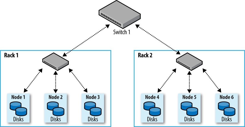
Figure 10-1. Typical two-level network architecture for a Hadoop cluster
Rack awareness
To get maximum performance out of Hadoop, it is important to configure Hadoop so that it knows the topology of your network. If your cluster runs on a single rack, then there is nothing more to do, since this is the default. However, for multirack clusters, you need to map nodes to racks. This allows Hadoop to prefer within-rack transfers (where there is more bandwidth available) to off-rack transfers when placing MapReduce tasks on nodes. HDFS will also be able to place replicas more intelligently to trade off performance and resilience.
Network locations such as nodes and racks are represented in a tree, which reflects the network “distance” between locations. The namenode uses the network location when determining where to place block replicas (see Network Topology and Hadoop); the MapReduce scheduler uses network location to determine where the closest replica is for input to a map task.
For the network in Figure 10-1, the rack topology is described by two network locations — say, /switch1/rack1 and /switch1/rack2. Because there is only one top-level switch in this cluster, the locations can be simplified to /rack1 and /rack2.
The Hadoop configuration must specify a map between node addresses and network locations. The map is described by a Java interface, DNSToSwitchMapping, whose signature is:
public interface DNSToSwitchMapping { public List
The names parameter is a list of IP addresses, and the return value is a list of corresponding network location strings. The net.topology.node.switch.mapping.impl configuration property defines an implementation of the DNSToSwitchMapping interface that the namenode and the resource manager use to resolve worker node network locations.
For the network in our example, we would map node1, node2, and node3 to /rack1, and node4, node5, and node6 to /rack2.
Most installations don’t need to implement the interface themselves, however, since the default implementation is ScriptBasedMapping, which runs a user-defined script to determine the mapping. The script’s location is controlled by the property net.topology.script.file.name. The script must accept a variable number of arguments that are the hostnames or IP addresses to be mapped, and it must emit the corresponding network locations to standard output, separated by whitespace. The Hadoop wiki has an example.
If no script location is specified, the default behavior is to map all nodes to a single network location, called /default-rack.
Cluster Setup and Installation
This section describes how to install and configure a basic Hadoop cluster from scratch using the Apache Hadoop distribution on a Unix operating system. It provides background information on the things you need to think about when setting up Hadoop. For a production installation, most users and operators should consider one of the Hadoop cluster management tools listed at the beginning of this chapter.
Installing Java
Hadoop runs on both Unix and Windows operating systems, and requires Java to be installed. For a production installation, you should select a combination of operating system, Java, and Hadoop that has been certified by the vendor of the Hadoop distribution you are using. There is also a page on the Hadoop wiki that lists combinations that community members have run with success.
Creating Unix User Accounts
It’s good practice to create dedicated Unix user accounts to separate the Hadoop processes from each other, and from other services running on the same machine. The HDFS, MapReduce, and YARN services are usually run as separate users, named hdfs, mapred, and yarn, respectively. They all belong to the same hadoop group.
Installing Hadoop
Download Hadoop from the Apache Hadoop releases page, and unpack the contents of the distribution in a sensible location, such as /usr/local (/opt is another standard choice; note that Hadoop should not be installed in a user’s home directory, as that may be an NFSmounted directory):
% cd /usr/local
% sudo tar xzf hadoop-x.y.z.tar.gz
You also need to change the owner of the Hadoop files to be the hadoop user and group:
% sudo chown -R hadoop:hadoop hadoop-x.y.z
It’s convenient to put the Hadoop binaries on the shell path too:
% export HADOOPHOME=/usr/local/hadoop-_x.y.z
% export PATH=$PATH:$HADOOP_HOME/bin:$HADOOP_HOME/sbin
Configuring SSH
The Hadoop control scripts (but not the daemons) rely on SSH to perform cluster-wide operations. For example, there is a script for stopping and starting all the daemons in the cluster. Note that the control scripts are optional — cluster-wide operations can be performed by other mechanisms, too, such as a distributed shell or dedicated Hadoop management applications.
To work seamlessly, SSH needs to be set up to allow passwordless login for the hdfs and yarn users from machines in the cluster.69] The simplest way to achieve this is to generate a public/private key pair and place it in an NFS location that is shared across the cluster.
First, generate an RSA key pair by typing the following. You need to do this twice, once as the hdfs user and once as the yarn user:
% ssh-keygen -t rsa -f ~/.ssh/id_rsa
Even though we want passwordless logins, keys without passphrases are not considered good practice (it’s OK to have an empty passphrase when running a local pseudodistributed cluster, as described in Appendix A), so we specify a passphrase when prompted for one. We use ssh-agent to avoid the need to enter a password for each connection.
The private key is in the file specified by the -f option, ~/.ssh/id_rsa, and the public key is stored in a file with the same name but with .pub appended, ~/.ssh/id_rsa.pub.
Next, we need to make sure that the public key is in the ~/.ssh/authorized_keys file on all the machines in the cluster that we want to connect to. If the users’ home directories are stored on an NFS filesystem, the keys can be shared across the cluster by typing the following (first as hdfs and then as yarn):
% cat ~/.ssh/id_rsa.pub >> ~/.ssh/authorized_keys
If the home directory is not shared using NFS, the public keys will need to be shared by some other means (such as ssh-copy-id).
Test that you can SSH from the master to a worker machine by making sure ssh-agent is running,70] and then run ssh-add to store your passphrase. You should be able to SSH to a worker without entering the passphrase again.
Configuring Hadoop
Hadoop must have its configuration set appropriately to run in distributed mode on a cluster. The important configuration settings to achieve this are discussed in Hadoop Configuration.
Formatting the HDFS Filesystem
Before it can be used, a brand-new HDFS installation needs to be formatted. The formatting process creates an empty filesystem by creating the storage directories and the initial versions of the namenode’s persistent data structures. Datanodes are not involved in the initial formatting process, since the namenode manages all of the filesystem’s metadata, and datanodes can join or leave the cluster dynamically. For the same reason, you don’t need to say how large a filesystem to create, since this is determined by the number of datanodes in the cluster, which can be increased as needed, long after the filesystem is formatted.
Formatting HDFS is a fast operation. Run the following command as the hdfs user:
% hdfs namenode -format
Starting and Stopping the Daemons
Hadoop comes with scripts for running commands and starting and stopping daemons across the whole cluster. To use these scripts (which can be found in the sbin directory), you need to tell Hadoop which machines are in the cluster. There is a file for this purpose, called slaves, which contains a list of the machine hostnames or IP addresses, one per line. The slaves file lists the machines that the datanodes and node managers should run on. It resides in Hadoop’s configuration directory, although it may be placed elsewhere (and given another name) by changing the HADOOPSLAVES setting in _hadoop-env.sh. Also, this file does not need to be distributed to worker nodes, since they are used only by the control scripts running on the namenode or resource manager.
The HDFS daemons are started by running the following command as the hdfs user:
% start-dfs.sh
The machine (or machines) that the namenode and secondary namenode run on is determined by interrogating the Hadoop configuration for their hostnames. For example, the script finds the namenode’s hostname by executing the following:
% hdfs getconf -namenodes
By default, this finds the namenode’s hostname from fs.defaultFS. In slightly more detail, the start-dfs.sh script does the following: Starts a namenode on each machine returned by executing hdfs getconf -
[71] namenodes
Starts a datanode on each machine listed in the slaves file
Starts a secondary namenode on each machine returned by executing hdfs getconf -
secondarynamenodes
The YARN daemons are started in a similar way, by running the following command as the yarn user on the machine hosting the resource manager:
% start-yarn.sh
In this case, the resource manager is always run on the machine from which the startyarn.sh script was run. More specifically, the script:
Starts a resource manager on the local machine
Starts a node manager on each machine listed in the slaves file
Also provided are stop-dfs.sh and stop-yarn.sh scripts to stop the daemons started by the corresponding start scripts.
These scripts start and stop Hadoop daemons using the hadoop-daemon.sh script (or the yarn-daemon.sh script, in the case of YARN). If you use the aforementioned scripts, you shouldn’t call hadoop-daemon.sh directly. But if you need to control Hadoop daemons from another system or from your own scripts, the hadoop-daemon.sh script is a good integration point. Likewise, hadoop-daemons.sh (with an “s”) is handy for starting the same daemon on a set of hosts.
Finally, there is only one MapReduce daemon — the job history server, which is started as follows, as the mapred user:
% mr-jobhistory-daemon.sh start historyserver
Creating User Directories
Once you have a Hadoop cluster up and running, you need to give users access to it. This involves creating a home directory for each user and setting ownership permissions on it:
% hadoop fs -mkdir /user/username
% hadoop fs -chown username:username /user/username
This is a good time to set space limits on the directory. The following sets a 1 TB limit on the given user directory:
% hdfs dfsadmin -setSpaceQuota 1t /user/username
Hadoop Configuration
There are a handful of files for controlling the configuration of a Hadoop installation; the most important ones are listed in Table 10-1.
Table 10-1. Hadoop configuration files
Filename Format Description
| hadoop-env.sh | Bash script | Environment variables that are used in the scripts to run Hadoop |
|---|---|---|
| mapred-env.sh | Bash script | Environment variables that are used in the scripts to run MapReduce (overrides variables set in hadoop-env.sh) |
| yarn-env.sh | Bash script | Environment variables that are used in the scripts to run YARN (overrides variables set in hadoop-env.sh) |
| core-site.xml | Hadoop configuration XML |
Configuration settings for Hadoop Core, such as I/O settings that are common to HDFS, MapReduce, and YARN |
| hdfs-site.xml | Hadoop configuration XML |
Configuration settings for HDFS daemons: the namenode, the secondary namenode, and the datanodes |
| mapred-site.xml | Hadoop configuration XML |
Configuration settings for MapReduce daemons: the job history server |
| yarn-site.xml | Hadoop configuration XML |
Configuration settings for YARN daemons: the resource manager, the web app proxy server, and the node managers |
| slaves | Plain text | A list of machines (one per line) that each run a datanode and a node manager |
| hadoop-metrics2 .properties | Java properties | Properties for controlling how metrics are published in Hadoop (see Metrics and JMX) |
| log4j.properties | Java properties | Properties for system logfiles, the namenode audit log, and the task log for the task JVM process (Hadoop Logs) |
| hadoop-policy.xml | Hadoop configuration XML |
Configuration settings for access control lists when running Hadoop in secure mode |
These files are all found in the etc/hadoop directory of the Hadoop distribution. The configuration directory can be relocated to another part of the filesystem (outside the Hadoop installation, which makes upgrades marginally easier) as long as daemons are started with the —config option (or, equivalently, with the HADOOP_CONF_DIR environment variable set) specifying the location of this directory on the local filesystem.
Configuration Management
Hadoop does not have a single, global location for configuration information. Instead, each Hadoop node in the cluster has its own set of configuration files, and it is up to administrators to ensure that they are kept in sync across the system. There are parallel shell tools that can help do this, such as dsh or pdsh. This is an area where Hadoop cluster management tools like Cloudera Manager and Apache Ambari really shine, since they take care of propagating changes across the cluster.
Hadoop is designed so that it is possible to have a single set of configuration files that are used for all master and worker machines. The great advantage of this is simplicity, both conceptually (since there is only one configuration to deal with) and operationally (as the Hadoop scripts are sufficient to manage a single configuration setup).
For some clusters, the one-size-fits-all configuration model breaks down. For example, if you expand the cluster with new machines that have a different hardware specification from the existing ones, you need a different configuration for the new machines to take advantage of their extra resources.
In these cases, you need to have the concept of a class of machine and maintain a separate configuration for each class. Hadoop doesn’t provide tools to do this, but there are several excellent tools for doing precisely this type of configuration management, such as Chef, Puppet, CFEngine, and Bcfg2.
For a cluster of any size, it can be a challenge to keep all of the machines in sync. Consider what happens if the machine is unavailable when you push out an update. Who ensures it gets the update when it becomes available? This is a big problem and can lead to divergent installations, so even if you use the Hadoop control scripts for managing Hadoop, it may be a good idea to use configuration management tools for maintaining the cluster. These tools are also excellent for doing regular maintenance, such as patching security holes and updating system packages.
Environment Settings
In this section, we consider how to set the variables in hadoop-env.sh. There are also analogous configuration files for MapReduce and YARN (but not for HDFS), called mapred-env.sh and yarn-env.sh, where variables pertaining to those components can be set. Note that the MapReduce and YARN files override the values set in hadoop-env.sh.
Java
The location of the Java implementation to use is determined by the JAVAHOME setting in _hadoop-env.sh or the JAVAHOME shell environment variable, if not set in _hadoop-env.sh. It’s a good idea to set the value in hadoop-env.sh, so that it is clearly defined in one place and to ensure that the whole cluster is using the same version of Java.
Memory heap size
By default, Hadoop allocates 1,000 MB (1 GB) of memory to each daemon it runs. This is controlled by the HADOOPHEAPSIZE setting in _hadoop-env.sh. There are also environment variables to allow you to change the heap size for a single daemon. For example, you can set YARNRESOURCEMANAGER_HEAPSIZE in _yarn-env.sh to override the heap size for the resource manager.
Surprisingly, there are no corresponding environment variables for HDFS daemons, despite it being very common to give the namenode more heap space. There is another way to set the namenode heap size, however; this is discussed in the following sidebar.
HOW MUCH MEMORY DOES A NAMENODE NEED?
A namenode can eat up memory, since a reference to every block of every file is maintained in memory. It’s difficult to give a precise formula because memory usage depends on the number of blocks per file, the filename length, and the number of directories in the filesystem; plus, it can change from one Hadoop release to another.
The default of 1,000 MB of namenode memory is normally enough for a few million files, but as a rule of thumb for sizing purposes, you can conservatively allow 1,000 MB per million blocks of storage.
For example, a 200-node cluster with 24 TB of disk space per node, a block size of 128 MB, and a replication factor of 3 has room for about 2 million blocks (or more): 200 × 24,000,000 MB ⁄ (128 MB × 3). So in this case, setting the namenode memory to 12,000 MB would be a good starting point.
You can increase the namenode’s memory without changing the memory allocated to other Hadoop daemons by setting HADOOPNAMENODE_OPTS in _hadoop-env.sh to include a JVM option for setting the memory size.
HADOOP_NAMENODE_OPTS allows you to pass extra options to the namenode’s JVM. So, for example, if you were using a Sun JVM, -Xmx2000m would specify that 2,000 MB of memory should be allocated to the namenode.
If you change the namenode’s memory allocation, don’t forget to do the same for the secondary namenode (using the
HADOOP_SECONDARYNAMENODE_OPTS variable), since its memory requirements are comparable to the primary namenode’s.
In addition to the memory requirements of the daemons, the node manager allocates containers to applications, so we need to factor these into the total memory footprint of a worker machine; see Memory settings in YARN and MapReduce.
System logfiles
System logfiles produced by Hadoop are stored in $HADOOP_HOME/logs by default. This can be changed using the HADOOPLOG_DIR setting in _hadoop-env.sh. It’s a good idea to change this so that logfiles are kept out of the directory that Hadoop is installed in. Changing this keeps logfiles in one place, even after the installation directory changes due to an upgrade. A common choice is /var/log/hadoop, set by including the following line in hadoop-env.sh: export HADOOPLOG_DIR=/var/log/hadoop
The log directory will be created if it doesn’t already exist. (If it does not exist, confirm that the relevant Unix Hadoop user has permission to create it.) Each Hadoop daemon running on a machine produces two logfiles. The first is the log output written via log4j. This file, whose name ends in .log, should be the first port of call when diagnosing problems because most application log messages are written here. The standard Hadoop log4j configuration uses a daily rolling file appender to rotate logfiles. Old logfiles are never deleted, so you should arrange for them to be periodically deleted or archived, so as to not run out of disk space on the local node.
The second logfile is the combined standard output and standard error log. This logfile, whose name ends in .out, usually contains little or no output, since Hadoop uses log4j for logging. It is rotated only when the daemon is restarted, and only the last five logs are retained. Old logfiles are suffixed with a number between 1 and 5, with 5 being the oldest file.
Logfile names (of both types) are a combination of the name of the user running the daemon, the daemon name, and the machine hostname. For example, _hadoop-hdfsdatanode-ip-10-45-174-112.log.2014-09-20 is the name of a logfile after it has been rotated. This naming structure makes it possible to archive logs from all machines in the cluster in a single directory, if needed, since the filenames are unique.
The username in the logfile name is actually the default for the HADOOPIDENT_STRING setting in _hadoop-env.sh. If you wish to give the Hadoop instance a different identity for the purposes of naming the logfiles, change HADOOP_IDENT_STRING to be the identifier you want.
SSH settings
The control scripts allow you to run commands on (remote) worker nodes from the master node using SSH. It can be useful to customize the SSH settings, for various reasons. For example, you may want to reduce the connection timeout (using the ConnectTimeout option) so the control scripts don’t hang around waiting to see whether a dead node is going to respond. Obviously, this can be taken too far. If the timeout is too low, then busy nodes will be skipped, which is bad.
Another useful SSH setting is StrictHostKeyChecking, which can be set to no to automatically add new host keys to the known hosts files. The default, ask, prompts the user to confirm that the key fingerprint has been verified, which is not a suitable setting in a large cluster environment.72]
To pass extra options to SSH, define the HADOOPSSH_OPTS environment variable in _hadoop-env.sh. See the ssh and ssh_config manual pages for more SSH settings.
Important Hadoop Daemon Properties
Hadoop has a bewildering number of configuration properties. In this section, we address the ones that you need to define (or at least understand why the default is appropriate) for any real-world working cluster. These properties are set in the Hadoop site files: coresite.xml, hdfs-site.xml, and yarn-site.xml. Typical instances of these files are shown in
Examples 10-1, 10-2, and 10-3.73] You can learn more about the format of Hadoop’s configuration files in The Configuration API.
To find the actual configuration of a running daemon, visit the /conf page on its web server. For example, http://__resource-manager-host:8088/conf shows the configuration that the resource manager is running with. This page shows the combined site and default configuration files that the daemon is running with, and also shows which file each property was picked up from.
Example 10-1. A typical core-site.xml configuration file
<?xml version=”1.0”?>
Example 10-2. A typical hdfs-site.xml configuration file
<?xml version=”1.0”?>
Example 10-3. A typical yarn-site.xml configuration file
<?xml version=”1.0”?>
HDFS
To run HDFS, you need to designate one machine as a namenode. In this case, the property fs.defaultFS is an HDFS filesystem URI whose host is the namenode’s hostname or IP address and whose port is the port that the namenode will listen on for RPCs. If no port is specified, the default of 8020 is used.
The fs.defaultFS property also doubles as specifying the default filesystem. The default filesystem is used to resolve relative paths, which are handy to use because they save typing (and avoid hardcoding knowledge of a particular namenode’s address). For example, with the default filesystem defined in Example 10-1, the relative URI /a/b is resolved to hdfs://namenode/a/b.
NOTE
If you are running HDFS, the fact that fs.defaultFS is used to specify both the HDFS namenode and the default filesystem means HDFS has to be the default filesystem in the server configuration. Bear in mind, however, that it is possible to specify a different filesystem as the default in the client configuration, for convenience.
For example, if you use both HDFS and S3 filesystems, then you have a choice of specifying either as the default in the client configuration, which allows you to refer to the default with a relative URI and the other with an absolute URI.
There are a few other configuration properties you should set for HDFS: those that set the storage directories for the namenode and for datanodes. The property dfs.namenode.name.dir specifies a list of directories where the namenode stores persistent filesystem metadata (the edit log and the filesystem image). A copy of each metadata file is stored in each directory for redundancy. It’s common to configure dfs.namenode.name.dir so that the namenode metadata is written to one or two local disks, as well as a remote disk, such as an NFS-mounted directory. Such a setup guards against failure of a local disk and failure of the entire namenode, since in both cases the files can be recovered and used to start a new namenode. (The secondary namenode takes only periodic checkpoints of the namenode, so it does not provide an up-to-date backup of the namenode.)
You should also set the dfs.datanode.data.dir property, which specifies a list of directories for a datanode to store its blocks in. Unlike the namenode, which uses multiple directories for redundancy, a datanode round-robins writes between its storage directories, so for performance you should specify a storage directory for each local disk. Read performance also benefits from having multiple disks for storage, because blocks will be spread across them and concurrent reads for distinct blocks will be correspondingly spread across disks.
TIP
For maximum performance, you should mount storage disks with the noatime option. This setting means that last accessed time information is not written on file reads, which gives significant performance gains.
Finally, you should configure where the secondary namenode stores its checkpoints of the filesystem. The dfs.namenode.checkpoint.dir property specifies a list of directories where the checkpoints are kept. Like the storage directories for the namenode, which keep redundant copies of the namenode metadata, the checkpointed filesystem image is stored in each checkpoint directory for redundancy.
Table 10-2 summarizes the important configuration properties for HDFS.
Table 10-2. Important HDFS daemon properties
Property name Type Default value Description
fs.defaultFS URI file:/// The default
filesystem. The URI defines the hostname and port that the
namenode’s RPC
server runs on. The default port is 8020. This property is set in core-site.xml.
| dfs.namenode.name.dir | Comma- separated directory names |
file://${hadoop.tmp.dir}/dfs/name | The list of directories where the namenode stores its persistent metadata. The namenode stores a copy of the metadata in each directory in the list. |
|
|---|---|---|---|---|
| dfs.datanode.data.dir | Comma- separated directory names |
file://${hadoop.tmp.dir}/dfs/data | A list of directories where the datanode stores blocks. Each block is stored in only one of these directories. | |
| dfs.namenode.checkpoint.dir Commaseparated directory names | file://${hadoop.tmp.dir}/dfs/namesecondary A list of directories where the secondary namenode stores checkpoints. It stores a copy of the checkpoint in each directory in the list. |
WARNING
Note that the storage directories for HDFS are under Hadoop’s temporary directory by default (this is configured via the hadoop.tmp.dir property, whose default is /tmp/hadoop-${user.name}). Therefore, it is critical that these properties are set so that data is not lost by the system when it clears out temporary directories.
YARN
To run YARN, you need to designate one machine as a resource manager. The simplest way to do this is to set the property yarn.resourcemanager.hostname to the hostname or IP address of the machine running the resource manager. Many of the resource manager’s server addresses are derived from this property. For example, yarn.resourcemanager.address takes the form of a host-port pair, and the host defaults to yarn.resourcemanager.hostname. In a MapReduce client configuration, this property is used to connect to the resource manager over RPC.
During a MapReduce job, intermediate data and working files are written to temporary local files. Because this data includes the potentially very large output of map tasks, you need to ensure that the yarn.nodemanager.local-dirs property, which controls the location of local temporary storage for YARN containers, is configured to use disk partitions that are large enough. The property takes a comma-separated list of directory names, and you should use all available local disks to spread disk I/O (the directories are used in round-robin fashion). Typically, you will use the same disks and partitions (but different directories) for YARN local storage as you use for datanode block storage, as governed by the dfs.datanode.data.dir property, which was discussed earlier.
Unlike MapReduce 1, YARN doesn’t have tasktrackers to serve map outputs to reduce tasks, so for this function it relies on shuffle handlers, which are long-running auxiliary services running in node managers. Because YARN is a general-purpose service, the MapReduce shuffle handlers need to be enabled explicitly in yarn-site.xml by setting the yarn.nodemanager.aux-services property to mapreduceshuffle.
Table 10-3 summarizes the important configuration properties for YARN. The resourcerelated settings are covered in more detail in the next sections.
_Table 10-3. Important YARN daemon properties
| Property name | Type Default value Description |
|---|---|
| yarn.resourcemanager.hostname | Hostname 0.0.0.0 The hostname of the machine the resource manager runs on. Abbreviated ${y.rm.hostname} below. |
| yarn.resourcemanager.address | Hostname ${y.rm.hostname}:8032 The hostname and port that the resource and port manager’s RPC server runs on. |
yarn.nodemanager.local-dirs Comma- ${hadoop.tmp.dir}/nm- A list of directories where node
separated local-dir managers allow containers to store directory intermediate data. The data is cleared names out when the application ends.
| yarn.nodemanager.aux-services | Comma- separated service names |
A list of auxiliary services run by the node manager. A service is implemented by the class defined by the property yarn.nodemanager.auxservices.service-name.class. By default, no auxiliary services are specified. |
|
|---|---|---|---|
yarn.nodemanager.resource.memory- int 8192 The amount of physical memory (in
mb MB) that may be allocated to containers
being run by the node manager.
| yarn.nodemanager.vmem-pmem-ratio | float | 2.1 | The ratio of virtual to physical memory for containers. Virtual memory usage may exceed the allocation by this amount. |
|---|---|---|---|
yarn.nodemanager.resource.cpu- int 8 The number of CPU cores that may be
vcores allocated to containers being run by the node manager.
Memory settings in YARN and MapReduce
YARN treats memory in a more fine-grained manner than the slot-based model used in MapReduce 1. Rather than specifying a fixed maximum number of map and reduce slots that may run on a node at once, YARN allows applications to request an arbitrary amount of memory (within limits) for a task. In the YARN model, node managers allocate memory from a pool, so the number of tasks that are running on a particular node depends on the sum of their memory requirements, and not simply on a fixed number of slots.
The calculation for how much memory to dedicate to a node manager for running containers depends on the amount of physical memory on the machine. Each Hadoop daemon uses 1,000 MB, so for a datanode and a node manager, the total is 2,000 MB. Set aside enough for other processes that are running on the machine, and the remainder can be dedicated to the node manager’s containers by setting the configuration property yarn.nodemanager.resource.memory-mb to the total allocation in MB. (The default is 8,192 MB, which is normally too low for most setups.)
The next step is to determine how to set memory options for individual jobs. There are two main controls: one for the size of the container allocated by YARN, and another for the heap size of the Java process run in the container.
Container sizes are determined by mapreduce.map.memory.mb and mapreduce.reduce.memory.mb; both default to 1,024 MB. These settings are used by the application master when negotiating for resources in the cluster, and also by the node manager, which runs and monitors the task containers. The heap size of the Java process is set by mapred.child.java.opts, and defaults to 200 MB. You can also set the Java options separately for map and reduce tasks (see Table 10-4).
Table 10-4. MapReduce job memory properties (set by the client)
Property name Type Default Description value
| mapreduce.map.memory.mb | int | 1024 | The amount of memory for map containers. |
|---|---|---|---|
| mapreduce.reduce.memory.mb | int | 1024 | The amount of memory for reduce containers. |
| mapred.child.java.opts | String | - Xmx200m |
The JVM options used to launch the container process that runs map and reduce tasks. In addition to memory settings, this property can include JVM properties for debugging, for example. |
| mapreduce.map.java.opts | String | - Xmx200m |
The JVM options used for the child process that runs map tasks. |
| mapreduce.reduce.java.opts | String | - Xmx200m |
The JVM options used for the child process that runs reduce tasks. |
For example, suppose mapred.child.java.opts is set to -Xmx800m and mapreduce.map.memory.mb is left at its default value of 1,024 MB. When a map task is run, the node manager will allocate a 1,024 MB container (decreasing the size of its pool by that amount for the duration of the task) and will launch the task JVM configured with an 800 MB maximum heap size. Note that the JVM process will have a larger memory footprint than the heap size, and the overhead will depend on such things as the native libraries that are in use, the size of the permanent generation space, and so on. The important thing is that the physical memory used by the JVM process, including any processes that it spawns, such as Streaming processes, does not exceed its allocation (1,024 MB). If a container uses more memory than it has been allocated, then it may be terminated by the node manager and marked as failed.
YARN schedulers impose a minimum or maximum on memory allocations. The default minimum is 1,024 MB (set by yarn.scheduler.minimum-allocation-mb), and the default maximum is 8,192 MB (set by yarn.scheduler.maximum-allocation-mb).
There are also virtual memory constraints that a container must meet. If a container’s virtual memory usage exceeds a given multiple of the allocated physical memory, the node manager may terminate the process. The multiple is expressed by the yarn.nodemanager.vmem-pmem-ratio property, which defaults to 2.1. In the example used earlier, the virtual memory threshold above which the task may be terminated is 2,150 MB, which is 2.1 × 1,024 MB.
When configuring memory parameters it’s very useful to be able to monitor a task’s actual memory usage during a job run, and this is possible via MapReduce task counters. The
counters PHYSICAL_MEMORY_BYTES, VIRTUAL_MEMORY_BYTES, and COMMITTED_HEAP_BYTES (described in Table 9-2) provide snapshot values of memory usage and are therefore suitable for observation during the course of a task attempt.
Hadoop also provides settings to control how much memory is used for MapReduce operations. These can be set on a per-job basis and are covered in Shuffle and Sort.
CPU settings in YARN and MapReduce
In addition to memory, YARN treats CPU usage as a managed resource, and applications can request the number of cores they need. The number of cores that a node manager can allocate to containers is controlled by the yarn.nodemanager.resource.cpu-vcores property. It should be set to the total number of cores on the machine, minus a core for each daemon process running on the machine (datanode, node manager, and any other long-running processes).
MapReduce jobs can control the number of cores allocated to map and reduce containers by setting mapreduce.map.cpu.vcores and mapreduce.reduce.cpu.vcores. Both default to 1, an appropriate setting for normal single-threaded MapReduce tasks, which can only saturate a single core.
WARNING
While the number of cores is tracked during scheduling (so a container won’t be allocated on a machine where there are no spare cores, for example), the node manager will not, by default, limit actual CPU usage of running containers. This means that a container can abuse its allocation by using more CPU than it was given, possibly starving other containers running on the same host. YARN has support for enforcing CPU limits using Linux cgroups. The node manager’s container executor class (yarn.nodemanager.container-executor.class) must be set to use the LinuxContainerExecutor class, which in turn must be configured to use cgroups (see the properties under yarn.nodemanager.linux-container-executor).
Hadoop Daemon Addresses and Ports
Hadoop daemons generally run both an RPC server for communication between daemons
(Table 10-5) and an HTTP server to provide web pages for human consumption (Table 106). Each server is configured by setting the network address and port number to listen on.
A port number of 0 instructs the server to start on a free port, but this is generally discouraged because it is incompatible with setting cluster-wide firewall policies.
In general, the properties for setting a server’s RPC and HTTP addresses serve double duty: they determine the network interface that the server will bind to, and they are used by clients or other machines in the cluster to connect to the server. For example, node managers use the yarn.resourcemanager.resource-tracker.address property to find the address of their resource manager.
It is often desirable for servers to bind to multiple network interfaces, but setting the network address to 0.0.0.0, which works for the server, breaks the second case, since the address is not resolvable by clients or other machines in the cluster. One solution is to have separate configurations for clients and servers, but a better way is to set the bind host for the server. By setting yarn.resourcemanager.hostname to the (externally resolvable) hostname or IP address and yarn.resourcemanager.bind-host to 0.0.0.0, you ensure that the resource manager will bind to all addresses on the machine, while at the same time providing a resolvable address for node managers and clients.
In addition to an RPC server, datanodes run a TCP/IP server for block transfers. The server address and port are set by the dfs.datanode.address property , which has a default value of 0.0.0.0:50010.
Table 10-5. RPC server properties
Property name Default value Description
fs.defaultFS file:/// When set to an HDFS URI, this property
determines the namenode’s RPC server address and port. The default port is 8020 if not specified.
| dfs.namenode.rpc-bind-host | The address the namenode’s RPC server will bind to. If not set (the default), the bind address is determined by fs.defaultFS. It can be set to 0.0.0.0 to make the namenode listen on all interfaces. | |
|---|---|---|
dfs.datanode.ipc.address 0.0.0.0:50020 The datanode’s RPC server address and port.
| mapreduce.jobhistory.address | 0.0.0.0:10020 | The job history server’s RPC server address and port. This is used by the client (typically outside the cluster) to query job history. |
|---|---|---|
| mapreduce.jobhistory.bind-host | The address the job history server’s RPC and HTTP servers will bind to. | |
| yarn.resourcemanager.hostname | 0.0.0.0 | The hostname of the machine the resource manager runs on. Abbreviated ${y.rm.hostname} below. |
yarn.resourcemanager.bind-host The address the resource manager’s RPC and
HTTP servers will bind to.
| yarn.resourcemanager.address | ${y.rm.hostname}:8032 The resource manager’s RPC server address and port. This is used by the client (typically outside the cluster) to communicate with the resource manager. |
|---|---|
yarn.resourcemanager.admin.address ${y.rm.hostname}:8033 The resource manager’s admin RPC server
address and port. This is used by the admin client (invoked with yarn rmadmin, typically run outside the cluster) to communicate with the resource manager.
| yarn.resourcemanager.scheduler.address | ${y.rm.hostname}:8030 The resource manager scheduler’s RPC server address and port. This is used by (incluster) application masters to communicate with the resource manager. |
|---|---|
yarn.resourcemanager.resource- ${y.rm.hostname}:8031 The resource manager resource tracker’s RPC tracker.address server address and port. This is used by (in-
cluster) node managers to communicate with the resource manager.
| yarn.nodemanager.hostname | 0.0.0.0 | The hostname of the machine the node manager runs on. Abbreviated ${y.nm.hostname} below. |
|---|---|---|
| yarn.nodemanager.bind-host | The address the node manager’s RPC and HTTP servers will bind to. | |
| yarn.nodemanager.address | ${y.nm.hostname}:0 | The node manager’s RPC server address and port. This is used by (in-cluster) application masters to communicate with node managers. |
| yarn.nodemanager.localizer.address | ${y.nm.hostname}:8040 The node manager localizer’s RPC server address and port. |
Table 10-6. HTTP server properties
Property name Default value Description
| dfs.namenode.http-address 0.0.0.0:50070 | The namenode’s HTTP server address and port. |
|---|---|
| dfs.namenode.http-bind-host | The address the namenode’s HTTP server will bind to. |
| dfs.namenode.secondary.http-address 0.0.0.0:50090 | The secondary namenode’s HTTP server address and port. |
| dfs.datanode.http.address 0.0.0.0:50075 | The datanode’s HTTP server address and port. (Note that the property name is inconsistent with the ones for the namenode.) |
mapreduce.jobhistory.webapp.address 0.0.0.0:19888 The MapReduce job history server’s address and
port. This property is set in mapred-site.xml.
| mapreduce.shuffle.port | 13562 | The shuffle handler’s HTTP port number. This is used for serving map outputs, and is not a useraccessible web UI. This property is set in mapred-site.xml. |
|---|---|---|
yarn.resourcemanager.webapp.address ${y.rm.hostname}:8088 The resource manager’s HTTP server address and port.
| yarn.nodemanager.webapp.address | ${y.nm.hostname}:8042 The node manager’s HTTP server address and port. |
|---|---|
| yarn.web-proxy.address | The web app proxy server’s HTTP server address and port. If not set (the default), then the web app proxy server will run in the resource manager process. |
There is also a setting for controlling which network interfaces the datanodes use as their
IP addresses (for HTTP and RPC servers). The relevant property is dfs.datanode.dns.interface, which is set to default to use the default network interface. You can set this explicitly to report the address of a particular interface (eth0, for example).
Other Hadoop Properties
This section discusses some other properties that you might consider setting.
Cluster membership
To aid in the addition and removal of nodes in the future, you can specify a file containing a list of authorized machines that may join the cluster as datanodes or node managers. The file is specified using the dfs.hosts and yarn.resourcemanager.nodes.include-path properties (for datanodes and node managers, respectively), and the corresponding dfs.hosts.exclude and yarn.resourcemanager.nodes.exclude-path properties specify the files used for decommissioning. See Commissioning and Decommissioning Nodes for further discussion.
Buffer size
Hadoop uses a buffer size of 4 KB (4,096 bytes) for its I/O operations. This is a conservative setting, and with modern hardware and operating systems, you will likely see performance benefits by increasing it; 128 KB (131,072 bytes) is a common choice. Set the value in bytes using the io.file.buffer.size property in core-site.xml.
HDFS block size
The HDFS block size is 128 MB by default, but many clusters use more (e.g., 256 MB, which is 268,435,456 bytes) to ease memory pressure on the namenode and to give mappers more data to work on. Use the dfs.blocksize property in hdfs-site.xml to specify the size in bytes.
Reserved storage space
By default, datanodes will try to use all of the space available in their storage directories. If you want to reserve some space on the storage volumes for non-HDFS use, you can set dfs.datanode.du.reserved to the amount, in bytes, of space to reserve.
Trash
Hadoop filesystems have a trash facility, in which deleted files are not actually deleted but rather are moved to a trash folder, where they remain for a minimum period before being permanently deleted by the system. The minimum period in minutes that a file will remain in the trash is set using the fs.trash.interval configuration property in core-site.xml. By default, the trash interval is zero, which disables trash.
Like in many operating systems, Hadoop’s trash facility is a user-level feature, meaning that only files that are deleted using the filesystem shell are put in the trash. Files deleted programmatically are deleted immediately. It is possible to use the trash programmatically, however, by constructing a Trash instance, then calling its moveToTrash() method with the Path of the file intended for deletion. The method returns a value indicating success; a value of false means either that trash is not enabled or that the file is already in the trash.
When trash is enabled, users each have their own trash directories called .Trash in their home directories. File recovery is simple: you look for the file in a subdirectory of .Trash _and move it out of the trash subtree.
HDFS will automatically delete files in trash folders, but other filesystems will not, so you have to arrange for this to be done periodically. You can _expunge the trash, which will delete files that have been in the trash longer than their minimum period, using the filesystem shell:
% hadoop fs -expunge
The Trash class exposes an expunge() method that has the same effect.
Job scheduler
Particularly in a multiuser setting, consider updating the job scheduler queue configuration to reflect your organizational needs. For example, you can set up a queue for each group using the cluster. See Scheduling in YARN.
Reduce slow start
By default, schedulers wait until 5% of the map tasks in a job have completed before scheduling reduce tasks for the same job. For large jobs, this can cause problems with cluster utilization, since they take up reduce containers while waiting for the map tasks to complete. Setting mapreduce.job.reduce.slowstart.completedmaps to a higher value, such as 0.80 (80%), can help improve throughput.
Short-circuit local reads
When reading a file from HDFS, the client contacts the datanode and the data is sent to the client via a TCP connection. If the block being read is on the same node as the client, then it is more efficient for the client to bypass the network and read the block data directly from the disk. This is termed a short-circuit local read, and can make applications like HBase perform better.
You can enable short-circuit local reads by setting dfs.client.read.shortcircuit to true. Short-circuit local reads are implemented using Unix domain sockets, which use a local path for client-datanode communication. The path is set using the property dfs.domain.socket.path, and must be a path that only the datanode user (typically hdfs) or root can create, such as /var/run/hadoop-hdfs/dn_socket.
Security
Early versions of Hadoop assumed that HDFS and MapReduce clusters would be used by a group of cooperating users within a secure environment. The measures for restricting access were designed to prevent accidental data loss, rather than to prevent unauthorized access to data. For example, the file permissions system in HDFS prevents one user from accidentally wiping out the whole filesystem because of a bug in a program, or by mistakenly typing hadoop fs -rmr /, but it doesn’t prevent a malicious user from assuming root’s identity to access or delete any data in the cluster.
In security parlance, what was missing was a secure authentication mechanism to assure Hadoop that the user seeking to perform an operation on the cluster is who he claims to be and therefore can be trusted. HDFS file permissions provide only a mechanism for authorization, which controls what a particular user can do to a particular file. For example, a file may be readable only by a certain group of users, so anyone not in that group is not authorized to read it. However, authorization is not enough by itself, because the system is still open to abuse via spoofing by a malicious user who can gain network access to the cluster.
It’s common to restrict access to data that contains personally identifiable information (such as an end user’s full name or IP address) to a small set of users (of the cluster) within the organization who are authorized to access such information. Less sensitive (or anonymized) data may be made available to a larger set of users. It is convenient to host a mix of datasets with different security levels on the same cluster (not least because it means the datasets with lower security levels can be shared). However, to meet regulatory requirements for data protection, secure authentication must be in place for shared clusters.
This is the situation that Yahoo! faced in 2009, which led a team of engineers there to implement secure authentication for Hadoop. In their design, Hadoop itself does not manage user credentials; instead, it relies on Kerberos, a mature open-source network authentication protocol, to authenticate the user. However, Kerberos doesn’t manage permissions. Kerberos says that a user is who she says she is; it’s Hadoop’s job to determine whether that user has permission to perform a given action.
There’s a lot to security in Hadoop, and this section only covers the highlights. For more, readers are referred to Hadoop Security by Ben Spivey and Joey Echeverria (O’Reilly, 2014).
Kerberos and Hadoop
At a high level, there are three steps that a client must take to access a service when using Kerberos, each of which involves a message exchange with a server:
1. Authentication. The client authenticates itself to the Authentication Server and receives a timestamped Ticket-Granting Ticket (TGT).
2. Authorization. The client uses the TGT to request a service ticket from the TicketGranting Server.
3. Service request. The client uses the service ticket to authenticate itself to the server that is providing the service the client is using. In the case of Hadoop, this might be
the namenode or the resource manager.
Together, the Authentication Server and the Ticket Granting Server form the Key Distribution Center (KDC). The process is shown graphically in Figure 10-2.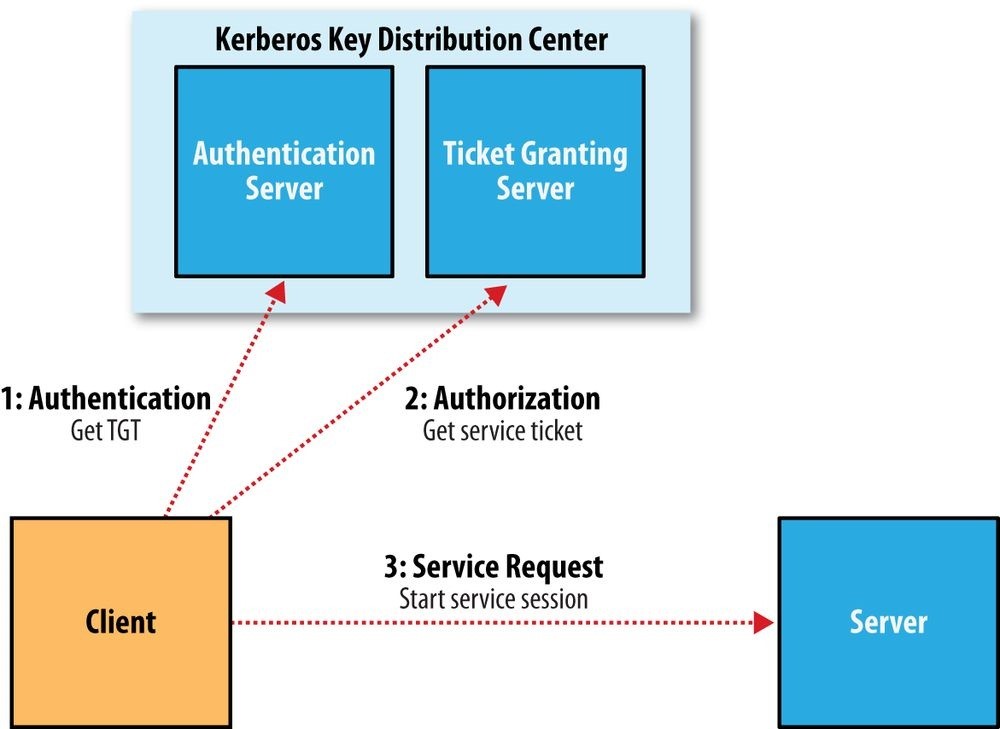
Figure 10-2. The three-step Kerberos ticket exchange protocol
The authorization and service request steps are not user-level actions; the client performs these steps on the user’s behalf. The authentication step, however, is normally carried out explicitly by the user using the kinit command, which will prompt for a password. However, this doesn’t mean you need to enter your password every time you run a job or access HDFS, since TGTs last for 10 hours by default (and can be renewed for up to a week). It’s common to automate authentication at operating system login time, thereby providing single sign-on to Hadoop.
In cases where you don’t want to be prompted for a password (for running an unattended MapReduce job, for example), you can create a Kerberos keytab file using the ktutil command. A keytab is a file that stores passwords and may be supplied to kinit with the -t option.
An example
Let’s look at an example of the process in action. The first step is to enable Kerberos authentication by setting the hadoop.security.authentication property in core-site.xml _to kerberos.74] The default setting is simple, which signifies that the old backwardcompatible (but insecure) behavior of using the operating system username to determine identity should be employed.
We also need to enable service-level authorization by setting hadoop.security.authorization to true in the same file. You may configure access control lists (ACLs) in the _hadoop-policy.xml configuration file to control which users and groups have permission to connect to each Hadoop service. Services are defined at the protocol level, so there are ones for MapReduce job submission, namenode communication, and so on. By default, all ACLs are set to , which means that all users have permission to access each service; however, on a real cluster you should lock the ACLs down to only those users and groups that should have access.
The format for an ACL is a comma-separated list of usernames, followed by whitespace, followed by a comma-separated list of group names. For example, the ACL preston,howard directors,inventors would authorize access to users named preston or howard, or in groups directors or inventors.
With Kerberos authentication turned on, let’s see what happens when we try to copy a local file to HDFS:
% hadoop fs -put quangle.txt .
10/07/03 15:44:58 WARN ipc.Client: Exception encountered while connecting to the server: javax.security.sasl.SaslException: GSS initiate failed [Caused by
GSSException: No valid credentials provided (Mechanism level: Failed to find any Kerberos tgt)]
Bad connection to FS. command aborted. exception: Call to localhost/
127.0.0.1:8020 failed on local exception: java.io.IOException: javax.security.sasl.SaslException: GSS initiate failed [Caused by GSSException:
No valid credentials provided
(Mechanism level: Failed to find any Kerberos tgt)]
The operation fails because we don’t have a Kerberos ticket. We can get one by authenticating to the KDC, using kinit:
% kinit
Password for hadoop-user@LOCALDOMAIN: password
% hadoop fs -put quangle.txt . % *hadoop fs -stat %n quangle.txt quangle.txt
And we see that the file is successfully written to HDFS. Notice that even though we carried out two filesystem commands, we only needed to call kinit once, since the Kerberos ticket is valid for 10 hours (use the klist command to see the expiry time of your tickets and kdestroy to invalidate your tickets). After we get a ticket, everything works just as it normally would.
Delegation Tokens
In a distributed system such as HDFS or MapReduce, there are many client-server interactions, each of which must be authenticated. For example, an HDFS read operation will involve multiple calls to the namenode and calls to one or more datanodes. Instead of using the three-step Kerberos ticket exchange protocol to authenticate each call, which would present a high load on the KDC on a busy cluster, Hadoop uses delegation tokens to allow later authenticated access without having to contact the KDC again. Delegation tokens are created and used transparently by Hadoop on behalf of users, so there’s no action you need to take as a user beyond using kinit to sign in, but it’s useful to have a basic idea of how they are used.
A delegation token is generated by the server (the namenode, in this case) and can be thought of as a shared secret between the client and the server. On the first RPC call to the namenode, the client has no delegation token, so it uses Kerberos to authenticate. As a part of the response, it gets a delegation token from the namenode. In subsequent calls it presents the delegation token, which the namenode can verify (since it generated it using a secret key), and hence the client is authenticated to the server.
When it wants to perform operations on HDFS blocks, the client uses a special kind of delegation token, called a block access token, that the namenode passes to the client in response to a metadata request. The client uses the block access token to authenticate itself to datanodes. This is possible only because the namenode shares its secret key used to generate the block access token with datanodes (sending it in heartbeat messages), so that they can verify block access tokens. Thus, an HDFS block may be accessed only by a client with a valid block access token from a namenode. This closes the security hole in unsecured Hadoop where only the block ID was needed to gain access to a block. This property is enabled by setting dfs.block.access.token.enable to true.
In MapReduce, job resources and metadata (such as JAR files, input splits, and configuration files) are shared in HDFS for the application master to access, and user code runs on the node managers and accesses files on HDFS (the process is explained in Anatomy of a MapReduce Job Run). Delegation tokens are used by these components to access HDFS during the course of the job. When the job has finished, the delegation tokens are invalidated.
Delegation tokens are automatically obtained for the default HDFS instance, but if your job needs to access other HDFS clusters, you can load the delegation tokens for these by setting the mapreduce.job.hdfs-servers job property to a comma-separated list of HDFS URIs.
Other Security Enhancements
Security has been tightened throughout the Hadoop stack to protect against unauthorized access to resources. The more notable features are listed here: Tasks can be run using the operating system account for the user who submitted the job, rather than the user running the node manager. This means that the operating system is used to isolate running tasks, so they can’t send signals to each other (to kill another user’s tasks, for example) and so local information, such as task data, is kept private via local filesystem permissions.
This feature is enabled by setting yarn.nodemanager.container-executor.class to
org.apache.hadoop.yarn.server.nodemanager.LinuxContainerExecutor.75] In addition, administrators need to ensure that each user is given an account on every node in the cluster (typically using LDAP). When tasks are run as the user who submitted the job, the distributed cache (see
Distributed Cache) is secure. Files that are world-readable are put in a shared cache (the insecure default); otherwise, they go in a private cache, readable only by the owner. Users can view and modify only their own jobs, not others. This is enabled by setting mapreduce.cluster.acls.enabled to true. There are two job configuration
properties, mapreduce.job.acl-view-job and mapreduce.job.acl-modify-job, which may be set to a comma-separated list of users to control who may view or modify a particular job.
The shuffle is secure, preventing a malicious user from requesting another user’s map outputs.
When appropriately configured, it’s no longer possible for a malicious user to run a rogue secondary namenode, datanode, or node manager that can join the cluster and potentially compromise data stored in the cluster. This is enforced by requiring daemons to authenticate with the master node they are connecting to.
To enable this feature, you first need to configure Hadoop to use a keytab previously generated with the ktutil command. For a datanode, for example, you would set the dfs.datanode.keytab.file property to the keytab filename and dfs.datanode.kerberos.principal to the username to use for the datanode. Finally, the ACL for the DataNodeProtocol (which is used by datanodes to communicate with the namenode) must be set in hadoop-policy.xml, by restricting security.datanode.protocol.acl to the datanode’s username.
A datanode may be run on a privileged port (one lower than 1024), so a client may be reasonably sure that it was started securely.
A task may communicate only with its parent application master, thus preventing an attacker from obtaining MapReduce data from another user’s job.
Various parts of Hadoop can be configured to encrypt network data, including RPC
(hadoop.rpc.protection), HDFS block transfers (dfs.encrypt.data.transfer), the
MapReduce shuffle (mapreduce.shuffle.ssl.enabled), and the web UIs
(hadokop.ssl.enabled). Work is ongoing to encrypt data “at rest,” too, so that HDFS blocks can be stored in encrypted form, for example.
Benchmarking a Hadoop Cluster
Is the cluster set up correctly? The best way to answer this question is empirically: run some jobs and confirm that you get the expected results. Benchmarks make good tests because you also get numbers that you can compare with other clusters as a sanity check on whether your new cluster is performing roughly as expected. And you can tune a cluster using benchmark results to squeeze the best performance out of it. This is often done with monitoring systems in place (see Monitoring), so you can see how resources are being used across the cluster.
To get the best results, you should run benchmarks on a cluster that is not being used by others. In practice, this will be just before it is put into service and users start relying on it. Once users have scheduled periodic jobs on a cluster, it is generally impossible to find a time when the cluster is not being used (unless you arrange downtime with users), so you should run benchmarks to your satisfaction before this happens.
Experience has shown that most hardware failures for new systems are hard drive failures. By running I/O-intensive benchmarks — such as the ones described next — you can “burn in” the cluster before it goes live.
Hadoop Benchmarks
Hadoop comes with several benchmarks that you can run very easily with minimal setup cost. Benchmarks are packaged in the tests JAR file, and you can get a list of them, with descriptions, by invoking the JAR file with no arguments:
% hadoop jar $HADOOP_HOME/share/hadoop/mapreduce/hadoop-mapreduce-*-tests.jar
Most of the benchmarks show usage instructions when invoked with no arguments. For example:
% hadoop jar $HADOOP_HOME/share/hadoop/mapreduce/hadoop-mapreduce-*-tests.jar \ TestDFSIO
TestDFSIO.1.7 Missing arguments.
Usage: TestDFSIO [genericOptions] -read [-random | -backward |
-skip [-skipSize Size]] | -write | -append | -clean [-compression codecClassName]
[-nrFiles N] [-size Size[B|KB|MB|GB|TB]] [-resFile resultFileName] [-bufferSize Bytes] [-rootDir]
Benchmarking MapReduce with TeraSort
Hadoop comes with a MapReduce program called TeraSort that does a total sort of its input.76] It is very useful for benchmarking HDFS and MapReduce together, as the full input dataset is transferred through the shuffle. The three steps are: generate some random data, perform the sort, then validate the results.
First, we generate some random data using teragen (found in the examples JAR file, not the tests one). It runs a map-only job that generates a specified number of rows of binary data. Each row is 100 bytes long, so to generate one terabyte of data using 1,000 maps, run the following (10t is short for 10 trillion):
% hadoop jar \
$HADOOP_HOME/share/hadoop/mapreduce/hadoop-mapreduce-examples-*.jar \ teragen -Dmapreduce.job.maps=1000 10t random-data Next, run terasort:
% hadoop jar \
$HADOOP_HOME/share/hadoop/mapreduce/hadoop-mapreduce-examples-*.jar \ terasort random-data sorted-data
The overall execution time of the sort is the metric we are interested in, but it’s instructive to watch the job’s progress via the web UI (http://__resource-manager-host:8088/), where you can get a feel for how long each phase of the job takes. Adjusting the parameters mentioned in Tuning a Job is a useful exercise, too.
As a final sanity check, we validate that the data in sorted-data is, in fact, correctly sorted:
% hadoop jar \
$HADOOP_HOME/share/hadoop/mapreduce/hadoop-mapreduce-examples-*.jar \ teravalidate sorted-data report
This command runs a short MapReduce job that performs a series of checks on the sorted data to check whether the sort is accurate. Any errors can be found in the report/part-r00000 output file.
Other benchmarks
There are many more Hadoop benchmarks, but the following are widely used:
TestDFSIO tests the I/O performance of HDFS. It does this by using a MapReduce job as a convenient way to read or write files in parallel.
MRBench (invoked with mrbench) runs a small job a number of times. It acts as a good counterpoint to TeraSort, as it checks whether small job runs are responsive. NNBench (invoked with nnbench) is useful for load-testing namenode hardware. Gridmix is a suite of benchmarks designed to model a realistic cluster workload by mimicking a variety of data-access patterns seen in practice. See the documentation in the distribution for how to run Gridmix. SWIM, or the Statistical Workload Injector for MapReduce, is a repository of real-life MapReduce workloads that you can use to generate representative test workloads for your system. TPCx-HS is a standardized benchmark based on TeraSort from the Transaction Processing Performance Council.
User Jobs
For tuning, it is best to include a few jobs that are representative of the jobs that your users run, so your cluster is tuned for these and not just for the standard benchmarks. If this is your first Hadoop cluster and you don’t have any user jobs yet, then either Gridmix or SWIM is a good substitute.
When running your own jobs as benchmarks, you should select a dataset for your user jobs and use it each time you run the benchmarks to allow comparisons between runs. When you set up a new cluster or upgrade a cluster, you will be able to use the same dataset to compare the performance with previous runs.
[68] ECC memory is strongly recommended, as several Hadoop users have reported seeing many checksum errors when using non-ECC memory on Hadoop clusters.
[69] The mapred user doesn’t use SSH, as in Hadoop 2 and later, the only MapReduce daemon is the job history server.
[70] See its man page for instructions on how to start ssh-agent.
[71] There can be more than one namenode when running HDFS HA.
[72] For more discussion on the security implications of SSH host keys, consult the article “SSH Host Key Protection” by Brian Hatch.
[73] Notice that there is no site file for MapReduce shown here. This is because the only MapReduce daemon is the job history server, and the defaults are sufficient.
[74] To use Kerberos authentication with Hadoop, you need to install, configure, and run a KDC (Hadoop does not come with one). Your organization may already have a KDC you can use (an Active Directory installation, for example); if not, you can set up an MIT Kerberos 5 KDC.
[75] LinuxTaskController uses a setuid executable called container-executor, found in the bin directory. You should ensure that this binary is owned by root and has the setuid bit set (with chmod +s).
[76] In 2008, TeraSort was used to break the world record for sorting 1 TB of data; see A Brief History of Apache Hadoop.
Chapter 11. Administering Hadoop
The previous chapter was devoted to setting up a Hadoop cluster. In this chapter, we look at the procedures to keep a cluster running smoothly.
HDFS
Persistent Data Structures
As an administrator, it is invaluable to have a basic understanding of how the components of HDFS — the namenode, the secondary namenode, and the datanodes — organize their persistent data on disk. Knowing which files are which can help you diagnose problems or spot that something is awry.
Namenode directory structure
A running namenode has a directory structure like this:
${dfs.namenode.name.dir}/
├── current
│ ├── VERSION
│ ├── edits0000000000000000001-0000000000000000019
│ ├── edits_inprogress_0000000000000000020
│ ├── fsimage_0000000000000000000
│ ├── fsimage_0000000000000000000.md5 │ ├── fsimage_0000000000000000019
│ ├── fsimage_0000000000000000019.md5
│ └── seen_txid └── in_use.lock
Recall from Chapter 10 that the dfs.namenode.name.dir property is a list of directories, with the same contents mirrored in each directory. This mechanism provides resilience, particularly if one of the directories is an NFS mount, as is recommended.
The _VERSION file is a Java properties file that contains information about the version of HDFS that is running. Here are the contents of a typical file:
#Mon Sep 29 09:54:36 BST 2014 namespaceID=1342387246 clusterID=CID-01b5c398-959c-4ea8-aae6-1e0d9bd8b142 cTime=0 storageType=NAMENODE blockpoolID=BP-526805057-127.0.0.1-1411980876842 layoutVersion=-57
The layoutVersion is a negative integer that defines the version of HDFS’s persistent data structures. This version number has no relation to the release number of the Hadoop distribution. Whenever the layout changes, the version number is decremented (for example, the version after −57 is −58). When this happens, HDFS needs to be upgraded, since a newer namenode (or datanode) will not operate if its storage layout is an older version. Upgrading HDFS is covered in Upgrades.
The namespaceID is a unique identifier for the filesystem namespace, which is created when the namenode is first formatted. The clusterID is a unique identifier for the HDFS cluster as a whole; this is important for HDFS federation (see HDFS Federation), where a cluster is made up of multiple namespaces and each namespace is managed by one namenode. The blockpoolID is a unique identifier for the block pool containing all the files in the namespace managed by this namenode.
The cTime property marks the creation time of the namenode’s storage. For newly formatted storage, the value is always zero, but it is updated to a timestamp whenever the filesystem is upgraded.
The storageType indicates that this storage directory contains data structures for a namenode.
The _in_use.lock file is a lock file that the namenode uses to lock the storage directory. This prevents another namenode instance from running at the same time with (and possibly corrupting) the same storage directory.
The other files in the namenode’s storage directory are the edits and fsimage files, and seen_txid. To understand what these files are for, we need to dig into the workings of the namenode a little more.
The filesystem image and edit log
When a filesystem client performs a write operation (such as creating or moving a file), the transaction is first recorded in the edit log. The namenode also has an in-memory representation of the filesystem metadata, which it updates after the edit log has been modified. The in-memory metadata is used to serve read requests.
Conceptually the edit log is a single entity, but it is represented as a number of files on disk. Each file is called a segment, and has the prefix edits and a suffix that indicates the transaction IDs contained in it. Only one file is open for writes at any one time
(edits_inprogress_0000000000000000020 in the preceding example), and it is flushed and
synced after every transaction before a success code is returned to the client. For namenodes that write to multiple directories, the write must be flushed and synced to every copy before returning successfully. This ensures that no transaction is lost due to machine failure.
Each fsimage file is a complete persistent checkpoint of the filesystem metadata. (The suffix indicates the last transaction in the image.) However, it is not updated for every filesystem write operation, because writing out the fsimage file, which can grow to be gigabytes in size, would be very slow. This does not compromise resilience because if the namenode fails, then the latest state of its metadata can be reconstructed by loading the latest fsimage from disk into memory, and then applying each of the transactions from the relevant point onward in the edit log. In fact, this is precisely what the namenode does when it starts up (see Safe Mode).
NOTE
Each fsimage file contains a serialized form of all the directory and file inodes in the filesystem. Each inode is an internal representation of a file or directory’s metadata and contains such information as the file’s replication level, modification and access times, access permissions, block size, and the blocks the file is made up of. For directories, the modification time, permissions, and quota metadata are stored.
An fsimage file does not record the datanodes on which the blocks are stored. Instead, the namenode keeps this mapping in memory, which it constructs by asking the datanodes for their block lists when they join the cluster and periodically afterward to ensure the namenode’s block mapping is up to date.
As described, the edit log would grow without bound (even if it was spread across several physical edits files). Though this state of affairs would have no impact on the system while the namenode is running, if the namenode were restarted, it would take a long time to apply each of the transactions in its (very long) edit log. During this time, the filesystem would be offline, which is generally undesirable.
The solution is to run the secondary namenode, whose purpose is to produce checkpoints of the primary’s in-memory filesystem metadata.77] The checkpointing process proceeds as follows (and is shown schematically in Figure 11-1 for the edit log and image files shown earlier):
1. The secondary asks the primary to roll its in-progress edits file, so new edits go to a new file. The primary also updates the seen_txid file in all its storage directories.
2. The secondary retrieves the latest fsimage and edits files from the primary (using
HTTP GET).
3. The secondary loads fsimage into memory, applies each transaction from edits, then creates a new merged fsimage file.
4. The secondary sends the new fsimage back to the primary (using HTTP PUT), and the primary saves it as a temporary .ckpt file.
5. The primary renames the temporary fsimage file to make it available.
At the end of the process, the primary has an up-to-date fsimage file and a short inprogress edits file (it is not necessarily empty, as it may have received some edits while the checkpoint was being taken). It is possible for an administrator to run this process manually while the namenode is in safe mode, using the hdfs dfsadmin -saveNamespace command.
This procedure makes it clear why the secondary has similar memory requirements to the primary (since it loads the fsimage into memory), which is the reason that the secondary needs a dedicated machine on large clusters.
The schedule for checkpointing is controlled by two configuration parameters. The secondary namenode checkpoints every hour (dfs.namenode.checkpoint.period in seconds), or sooner if the edit log has reached one million transactions since the last checkpoint (dfs.namenode.checkpoint.txns), which it checks every minute (dfs.namenode.checkpoint.check.period in seconds).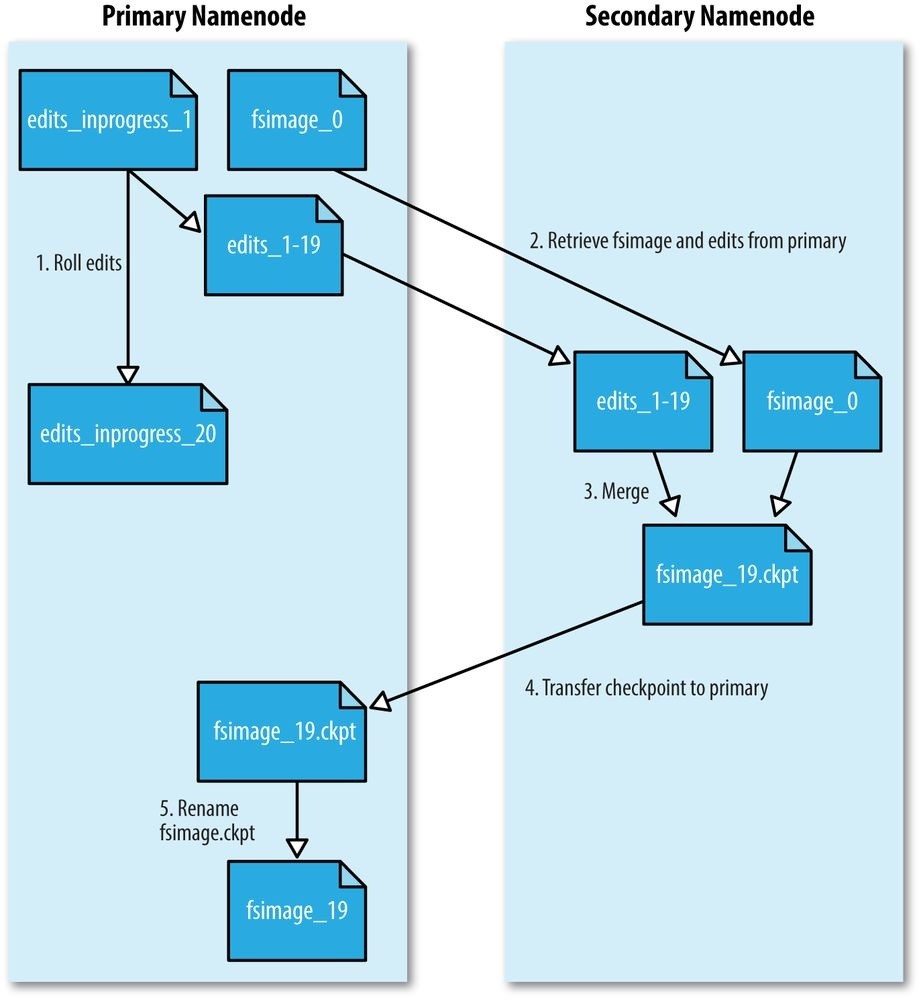
Figure 11-1. The checkpointing process
Secondary namenode directory structure
The layout of the secondary’s checkpoint directory (dfs.namenode.checkpoint.dir) is identical to the namenode’s. This is by design, since in the event of total namenode failure (when there are no recoverable backups, even from NFS), it allows recovery from a secondary namenode. This can be achieved either by copying the relevant storage directory to a new namenode or, if the secondary is taking over as the new primary namenode, by using the -importCheckpoint option when starting the namenode daemon. The -importCheckpoint option will load the namenode metadata from the latest checkpoint in the directory defined by the dfs.namenode.checkpoint.dir property, but only if there is no metadata in the dfs.namenode.name.dir directory, to ensure that there is no risk of overwriting precious metadata.
Datanode directory structure
Unlike namenodes, datanodes do not need to be explicitly formatted, because they create their storage directories automatically on startup. Here are the key files and directories:
${dfs.datanode.data.dir}/
├── current
│ ├── BP-526805057-127.0.0.1-1411980876842
│ │ └── current
│ │ ├── VERSION
│ │ ├── finalized
│ │ │ ├── blk1073741825
│ │ │ ├── blk10737418251001.meta │ │ │ ├── blk_1073741826
│ │ │ └── blk_1073741826_1002.meta
│ │ └── rbw
│ └── VERSION
└── in_use.lock
HDFS blocks are stored in files with a _blk prefix; they consist of the raw bytes of a portion of the file being stored. Each block has an associated metadata file with a .meta suffix. It is made up of a header with version and type information, followed by a series of checksums for sections of the block.
Each block belongs to a block pool, and each block pool has its own storage directory that is formed from its ID (it’s the same block pool ID from the namenode’s _VERSION file).
When the number of blocks in a directory grows to a certain size, the datanode creates a new subdirectory in which to place new blocks and their accompanying metadata. It creates a new subdirectory every time the number of blocks in a directory reaches 64 (set by the dfs.datanode.numblocks configuration property). The effect is to have a tree with high fan-out, so even for systems with a very large number of blocks, the directories will be only a few levels deep. By taking this measure, the datanode ensures that there is a manageable number of files per directory, which avoids the problems that most operating systems encounter when there are a large number of files (tens or hundreds of thousands) in a single directory.
If the configuration property dfs.datanode.data.dir specifies multiple directories on different drives, blocks are written in a round-robin fashion. Note that blocks are not replicated on each drive on a single datanode; instead, block replication is across distinct datanodes.
Safe Mode
When the namenode starts, the first thing it does is load its image file (fsimage) into memory and apply the edits from the edit log. Once it has reconstructed a consistent inmemory image of the filesystem metadata, it creates a new fsimage file (effectively doing the checkpoint itself, without recourse to the secondary namenode) and an empty edit log. During this process, the namenode is running in safe mode, which means that it offers only a read-only view of the filesystem to clients.
WARNING
Strictly speaking, in safe mode, only filesystem operations that access the filesystem metadata (such as producing a directory listing) are guaranteed to work. Reading a file will work only when the blocks are available on the current set of datanodes in the cluster, and file modifications (writes, deletes, or renames) will always fail.
Recall that the locations of blocks in the system are not persisted by the namenode; this information resides with the datanodes, in the form of a list of the blocks each one is storing. During normal operation of the system, the namenode has a map of block locations stored in memory. Safe mode is needed to give the datanodes time to check in to the namenode with their block lists, so the namenode can be informed of enough block locations to run the filesystem effectively. If the namenode didn’t wait for enough datanodes to check in, it would start the process of replicating blocks to new datanodes, which would be unnecessary in most cases (because it only needed to wait for the extra datanodes to check in) and would put a great strain on the cluster’s resources. Indeed, while in safe mode, the namenode does not issue any block-replication or deletion instructions to datanodes.
Safe mode is exited when the minimal replication condition is reached, plus an extension time of 30 seconds. The minimal replication condition is when 99.9% of the blocks in the whole filesystem meet their minimum replication level (which defaults to 1 and is set by dfs.namenode.replication.min; see Table 11-1).
When you are starting a newly formatted HDFS cluster, the namenode does not go into safe mode, since there are no blocks in the system.
Table 11-1. Safe mode properties
Property name Type Default Description
value
dfs.namenode.replication.min int 1 The minimum number of replicas that have
to be written for a write to be successful.
| dfs.namenode.safemode.threshold-pct | float | 0.999 | The proportion of blocks in the system that must meet the minimum replication level defined by dfs.namenode.replication.min before the namenode will exit safe mode. Setting this value to 0 or less forces the namenode not to start in safe mode. Setting this value to more than 1 means the namenode never exits safe mode. |
|---|---|---|---|
dfs.namenode.safemode.extension int 30000 The time, in milliseconds, to extend safe
mode after the minimum replication condition defined by
dfs.namenode.safemode.threshold-pct
has been satisfied. For small clusters (tens of nodes), it can be set to 0.
Entering and leaving safe mode
To see whether the namenode is in safe mode, you can use the dfsadmin command:
% hdfs dfsadmin -safemode get Safe mode is ON
The front page of the HDFS web UI provides another indication of whether the namenode is in safe mode.
Sometimes you want to wait for the namenode to exit safe mode before carrying out a command, particularly in scripts. The wait option achieves this:
% hdfs dfsadmin -safemode wait
# command to read or write a file
An administrator has the ability to make the namenode enter or leave safe mode at any time. It is sometimes necessary to do this when carrying out maintenance on the cluster or after upgrading a cluster, to confirm that data is still readable. To enter safe mode, use the following command:
% hdfs dfsadmin -safemode enter Safe mode is ON
You can use this command when the namenode is still in safe mode while starting up to ensure that it never leaves safe mode. Another way of making sure that the namenode stays in safe mode indefinitely is to set the property dfs.namenode.safemode.thresholdpct to a value over 1.
You can make the namenode leave safe mode by using the following:
% hdfs dfsadmin -safemode leave Safe mode is OFF
Audit Logging
HDFS can log all filesystem access requests, a feature that some organizations require for auditing purposes. Audit logging is implemented using log4j logging at the INFO level. In the default configuration it is disabled, but it’s easy to enable by adding the following line to hadoop-env.sh: export HDFSAUDIT_LOGGER=”INFO,RFAAUDIT”
A log line is written to the audit log (_hdfs-audit.log) for every HDFS event. Here’s an example for a list status request on /user/tom:
2014-09-30 21:35:30,484 INFO FSNamesystem.audit: allowed=true ugi=tom
(auth:SIMPLE) ip=/127.0.0.1 cmd=listStatus src=/user/tom dst=null perm=null proto=rpc
Tools dfsadmin
The dfsadmin tool is a multipurpose tool for finding information about the state of HDFS, as well as for performing administration operations on HDFS. It is invoked as hdfs dfsadmin and requires superuser privileges.
Some of the available commands to dfsadmin are described in Table 11-2. Use the -help command to get more information.
Table 11-2. dfsadmin commands
Command Description
| -help | Shows help for a given command, or all commands if no command is specified. |
|---|---|
| -report | Shows filesystem statistics (similar to those shown in the web UI) and information on connected datanodes. |
| -metasave | Dumps information to a file in Hadoop’s log directory about blocks that are being replicated or deleted, as well as a list of connected datanodes. |
| -safemode | Changes or queries the state of safe mode. See Safe Mode. |
| -saveNamespace | Saves the current in-memory filesystem image to a new fsimage file and resets the edits file. This operation may be performed only in safe mode. |
| -fetchImage | Retrieves the latest fsimage from the namenode and saves it in a local file. |
| -refreshNodes | Updates the set of datanodes that are permitted to connect to the namenode. See Commissioning and Decommissioning Nodes. |
| -upgradeProgress | Gets information on the progress of an HDFS upgrade or forces an upgrade to proceed. See Upgrades. |
-finalizeUpgrade Removes the previous version of the namenode and datanode storage directories. Used after an upgrade has been applied and the cluster is running successfully on the new version. See Upgrades.
| -setQuota | Sets directory quotas. Directory quotas set a limit on the number of names (files or directories) in the directory tree. Directory quotas are useful for preventing users from creating large numbers of small files, a measure that helps preserve the namenode’s memory (recall that accounting information for every file, directory, and block in the filesystem is stored in memory). |
|---|---|
-clrQuota Clears specified directory quotas.
| -setSpaceQuota | Sets space quotas on directories. Space quotas set a limit on the size of files that may be stored in a directory tree. They are useful for giving users a limited amount of storage. |
|---|---|
| -clrSpaceQuota | Clears specified space quotas. |
| - refreshServiceAcl |
Refreshes the namenode’s service-level authorization policy file. |
| -allowSnapshot | Allows snapshot creation for the specified directory. |
| -disallowSnapshot | Disallows snapshot creation for the specified directory. |
Filesystem check (fsck)
Hadoop provides an fsck utility for checking the health of files in HDFS. The tool looks for blocks that are missing from all datanodes, as well as under- or over-replicated blocks. Here is an example of checking the whole filesystem for a small cluster:
% hdfs fsck /
………………….Status: HEALTHY
Total size: 511799225 B
Total dirs: 10
Total files: 22
| Total blocks (validated): | 22 (avg. block size 23263601 B) |
|---|---|
| Minimally replicated blocks: | 22 (100.0 %) |
| Over-replicated blocks: | 0 (0.0 %) |
| Under-replicated blocks: | 0 (0.0 %) |
| Mis-replicated blocks: | 0 (0.0 %) |
| Default replication factor: | 3 |
| Average block replication: | 3.0 |
| Corrupt blocks: | 0 |
| Missing replicas: | 0 (0.0 %) |
| Number of data-nodes: | 4 |
| Number of racks: | 1 |
The filesystem under path ‘/‘ is HEALTHY fsck recursively walks the filesystem namespace, starting at the given path (here the filesystem root), and checks the files it finds. It prints a dot for every file it checks. To check a file, fsck retrieves the metadata for the file’s blocks and looks for problems or inconsistencies. Note that fsck retrieves all of its information from the namenode; it does not communicate with any datanodes to actually retrieve any block data.
Most of the output from fsck is self-explanatory, but here are some of the conditions it looks for:
Over-replicated blocks
These are blocks that exceed their target replication for the file they belong to.
Normally, over-replication is not a problem, and HDFS will automatically delete excess replicas.
Under-replicated blocks
These are blocks that do not meet their target replication for the file they belong to. HDFS will automatically create new replicas of under-replicated blocks until they meet the target replication. You can get information about the blocks being replicated (or waiting to be replicated) using hdfs dfsadmin -metasave.
Misreplicated blocks
These are blocks that do not satisfy the block replica placement policy (see Replica Placement). For example, for a replication level of three in a multirack cluster, if all three replicas of a block are on the same rack, then the block is misreplicated because the replicas should be spread across at least two racks for resilience. HDFS will automatically re-replicate misreplicated blocks so that they satisfy the rack placement policy.
Corrupt blocks
These are blocks whose replicas are all corrupt. Blocks with at least one noncorrupt replica are not reported as corrupt; the namenode will replicate the noncorrupt replica until the target replication is met.
Missing replicas
These are blocks with no replicas anywhere in the cluster.
Corrupt or missing blocks are the biggest cause for concern, as they mean data has been lost. By default, fsck leaves files with corrupt or missing blocks, but you can tell it to perform one of the following actions on them: Move the affected files to the /lost+found directory in HDFS, using the -move option. Files are broken into chains of contiguous blocks to aid any salvaging efforts you may attempt. Delete the affected files, using the -delete option. Files cannot be recovered after being deleted.
Finding the blocks for a file
The fsck tool provides an easy way to find out which blocks are in any particular file. For example:
% hdfs fsck /user/tom/part-00007 -files -blocks -racks
/user/tom/part-00007 25582428 bytes, 1 block(s): OK
0. blk-3724870485760122836_1035 len=25582428 repl=3 [/default-rack/10.251.43.2:
50010,/default-rack/10.251.27.178:50010, /default-rack/10.251.123.163:50010]
This says that the file /user/tom/part-00007 is made up of one block and shows the datanodes where the block is located. The _fsck options used are as follows:
The -files option shows the line with the filename, size, number of blocks, and its health (whether there are any missing blocks).
The -blocks option shows information about each block in the file, one line per block. The -racks option displays the rack location and the datanode addresses for each block.
Running hdfs fsck without any arguments displays full usage instructions.
Datanode block scanner
Every datanode runs a block scanner, which periodically verifies all the blocks stored on the datanode. This allows bad blocks to be detected and fixed before they are read by clients. The scanner maintains a list of blocks to verify and scans them one by one for checksum errors. It employs a throttling mechanism to preserve disk bandwidth on the datanode.
Blocks are verified every three weeks to guard against disk errors over time (this period is controlled by the dfs.datanode.scan.period.hours property, which defaults to 504 hours). Corrupt blocks are reported to the namenode to be fixed.
You can get a block verification report for a datanode by visiting the datanode’s web interface at http://__datanode:50075/blockScannerReport. Here’s an example of a report, which should be self-explanatory:
Total Blocks : 21131
Verified in last hour : 70
Verified in last day : 1767
Verified in last week : 7360
Verified in last four weeks : 20057
Verified in SCANPERIOD : 20057
Not yet verified : 1074
Verified since restart : 35912
Scans since restart : 6541
Scan errors since restart : 0
Transient scan errors : 0
Current scan rate limit KBps : 1024
Progress this period : 109%
Time left in cur period : 53.08%
If you specify the listblocks parameter, _http://__datanode:50075/blockScannerReport? listblocks, the report is preceded by a list of all the blocks on the datanode along with their latest verification status. Here is a snippet of the block list (lines are split to fit the page):
blk_6035596358209321442 : status : ok type : none scan time :
0 not yet verified blk_3065580480714947643 : status : ok type : remote scan time :
1215755306400 2008-07-11 05:48:26,400 blk_8729669677359108508 : status : ok type : local scan time :
1215755727345 2008-07-11 05:55:27,345
The first column is the block ID, followed by some key-value pairs. The status can be one of failed or ok, according to whether the last scan of the block detected a checksum error. The type of scan is local if it was performed by the background thread, remote if it was performed by a client or a remote datanode, or none if a scan of this block has yet to be made. The last piece of information is the scan time, which is displayed as the number of milliseconds since midnight on January 1, 1970, and also as a more readable value.
Balancer
Over time, the distribution of blocks across datanodes can become unbalanced. An unbalanced cluster can affect locality for MapReduce, and it puts a greater strain on the highly utilized datanodes, so it’s best avoided.
The balancer program is a Hadoop daemon that redistributes blocks by moving them from overutilized datanodes to underutilized datanodes, while adhering to the block replica placement policy that makes data loss unlikely by placing block replicas on different racks (see Replica Placement). It moves blocks until the cluster is deemed to be balanced, which means that the utilization of every datanode (ratio of used space on the node to total capacity of the node) differs from the utilization of the cluster (ratio of used space on the cluster to total capacity of the cluster) by no more than a given threshold percentage. You can start the balancer with:
% start-balancer.sh
The -threshold argument specifies the threshold percentage that defines what it means for the cluster to be balanced. The flag is optional; if omitted, the threshold is 10%. At any one time, only one balancer may be running on the cluster.
The balancer runs until the cluster is balanced, it cannot move any more blocks, or it loses contact with the namenode. It produces a logfile in the standard log directory, where it writes a line for every iteration of redistribution that it carries out. Here is the output from a short run on a small cluster (slightly reformatted to fit the page):
Time Stamp Iteration# Bytes Already Moved …Left To Move …Being Moved
Mar 18, 2009 5:23:42 PM 0 0 KB 219.21 MB 150.29 MB Mar 18, 2009 5:27:14 PM 1 195.24 MB 22.45 MB 150.29 MB
The cluster is balanced. Exiting…
Balancing took 6.072933333333333 minutes
The balancer is designed to run in the background without unduly taxing the cluster or interfering with other clients using the cluster. It limits the bandwidth that it uses to copy a block from one node to another. The default is a modest 1 MB/s, but this can be changed by setting the dfs.datanode.balance.bandwidthPerSec property in hdfs-site.xml, specified in bytes.
Monitoring
Monitoring is an important part of system administration. In this section, we look at the monitoring facilities in Hadoop and how they can hook into external monitoring systems.
The purpose of monitoring is to detect when the cluster is not providing the expected level of service. The master daemons are the most important to monitor: the namenodes (primary and secondary) and the resource manager. Failure of datanodes and node managers is to be expected, particularly on larger clusters, so you should provide extra capacity so that the cluster can tolerate having a small percentage of dead nodes at any time.
In addition to the facilities described next, some administrators run test jobs on a periodic basis as a test of the cluster’s health.
Logging
All Hadoop daemons produce logfiles that can be very useful for finding out what is happening in the system. System logfiles explains how to configure these files.
Setting log levels
When debugging a problem, it is very convenient to be able to change the log level temporarily for a particular component in the system.
Hadoop daemons have a web page for changing the log level for any log4j log name, which can be found at /logLevel in the daemon’s web UI. By convention, log names in Hadoop correspond to the names of the classes doing the logging, although there are exceptions to this rule, so you should consult the source code to find log names.
It’s also possible to enable logging for all packages that start with a given prefix. For example, to enable debug logging for all classes related to the resource manager, we would visit the its web UI at http://__resource-manager-host:8088/logLevel and set the log name org.apache.hadoop.yarn.server.resourcemanager to level DEBUG.
The same thing can be achieved from the command line as follows:
% hadoop daemonlog -setlevel resource-manager-host:8088 \ org.apache.hadoop.yarn.server.resourcemanager DEBUG
Log levels changed in this way are reset when the daemon restarts, which is usually what you want. However, to make a persistent change to a log level, you can simply change the log4j.properties file in the configuration directory. In this case, the line to add is: log4j.logger.org.apache.hadoop.yarn.server.resourcemanager=DEBUG
Getting stack traces
Hadoop daemons expose a web page (/stacks in the web UI) that produces a thread dump for all running threads in the daemon’s JVM. For example, you can get a thread dump for a resource manager from http://__resource-manager-host:8088/stacks.
Metrics and JMX
The Hadoop daemons collect information about events and measurements that are collectively known as metrics. For example, datanodes collect the following metrics (and many more): the number of bytes written, the number of blocks replicated, and the number of read requests from clients (both local and remote).
Metrics belong to a context; “dfs,” “mapred,” “yarn,” and “rpc” are examples of different contexts. Hadoop daemons usually collect metrics under several contexts. For example, datanodes collect metrics for the “dfs” and “rpc” contexts.
HOW DO METRICS DIFFER FROM COUNTERS?
The main difference is their scope: metrics are collected by Hadoop daemons, whereas counters (see Counters) are collected for MapReduce tasks and aggregated for the whole job. They have different audiences, too: broadly speaking, metrics are for administrators, and counters are for MapReduce users.
The way they are collected and aggregated is also different. Counters are a MapReduce feature, and the MapReduce system ensures that counter values are propagated from the task JVMs where they are produced back to the application master, and finally back to the client running the MapReduce job. (Counters are propagated via RPC heartbeats; see Progress and Status Updates.) Both the task process and the application master perform aggregation.
The collection mechanism for metrics is decoupled from the component that receives the updates, and there are various pluggable outputs, including local files, Ganglia, and JMX. The daemon collecting the metrics performs aggregation on them before they are sent to the output.
All Hadoop metrics are published to JMX (Java Management Extensions), so you can use standard JMX tools like JConsole (which comes with the JDK) to view them. For remote monitoring, you must set the JMX system property com.sun.management.jmxremote.port (and others for security) to allow access. To do this for the namenode, say, you would set the following in hadoop-env.sh:
HADOOPNAMENODE_OPTS=”-Dcom.sun.management.jmxremote.port=8004”
You can also view JMX metrics (in JSON format) gathered by a particular Hadoop daemon by connecting to its /jmx web page. This is handy for debugging. For example, you can view namenode metrics at _http://__namenode-host:50070/jmx.
Hadoop comes with a number of metrics sinks for publishing metrics to external systems, such as local files or the Ganglia monitoring system. Sinks are configured in the hadoopmetrics2.properties file; see that file for sample configuration settings.
Maintenance
Routine Administration Procedures
Metadata backups
If the namenode’s persistent metadata is lost or damaged, the entire filesystem is rendered unusable, so it is critical that backups are made of these files. You should keep multiple copies of different ages (one hour, one day, one week, and one month, say) to protect against corruption, either in the copies themselves or in the live files running on the namenode.
A straightforward way to make backups is to use the dfsadmin command to download a copy of the namenode’s most recent fsimage:
% hdfs dfsadmin -fetchImage fsimage.backup
You can write a script to run this command from an offsite location to store archive copies of the fsimage. The script should additionally test the integrity of the copy. This can be done by starting a local namenode daemon and verifying that it has successfully read the fsimage and edits files into memory (by scanning the namenode log for the appropriate success message, for example).78]
Data backups
Although HDFS is designed to store data reliably, data loss can occur, just like in any storage system; thus, a backup strategy is essential. With the large data volumes that Hadoop can store, deciding what data to back up and where to store it is a challenge. The key here is to prioritize your data. The highest priority is the data that cannot be regenerated and that is critical to the business; however, data that is either straightforward to regenerate or essentially disposable because it is of limited business value is the lowest priority, and you may choose not to make backups of this low-priority data.
WARNING
Do not make the mistake of thinking that HDFS replication is a substitute for making backups. Bugs in HDFS can cause replicas to be lost, and so can hardware failures. Although Hadoop is expressly designed so that hardware failure is very unlikely to result in data loss, the possibility can never be completely ruled out, particularly when combined with software bugs or human error.
When it comes to backups, think of HDFS in the same way as you would RAID. Although the data will survive the loss of an individual RAID disk, it may not survive if the RAID controller fails or is buggy (perhaps overwriting some data), or the entire array is damaged.
It’s common to have a policy for user directories in HDFS. For example, they may have space quotas and be backed up nightly. Whatever the policy, make sure your users know what it is, so they know what to expect.
The distcp tool is ideal for making backups to other HDFS clusters (preferably running on a different version of the software, to guard against loss due to bugs in HDFS) or other Hadoop filesystems (such as S3) because it can copy files in parallel. Alternatively, you can employ an entirely different storage system for backups, using one of the methods for exporting data from HDFS described in Hadoop Filesystems.
HDFS allows administrators and users to take snapshots of the filesystem. A snapshot is a read-only copy of a filesystem subtree at a given point in time. Snapshots are very efficient since they do not copy data; they simply record each file’s metadata and block list, which is sufficient to reconstruct the filesystem contents at the time the snapshot was taken.
Snapshots are not a replacement for data backups, but they are a useful tool for point-intime data recovery for files that were mistakenly deleted by users. You might have a policy of taking periodic snapshots and keeping them for a specific period of time according to age. For example, you might keep hourly snapshots for the previous day and daily snapshots for the previous month.
Filesystem check (fsck)
It is advisable to run HDFS’s fsck tool regularly (i.e., daily) on the whole filesystem to proactively look for missing or corrupt blocks. See Filesystem check (fsck).
Filesystem balancer
Run the balancer tool (see Balancer) regularly to keep the filesystem datanodes evenly balanced.
Commissioning and Decommissioning Nodes
As an administrator of a Hadoop cluster, you will need to add or remove nodes from time to time. For example, to grow the storage available to a cluster, you commission new nodes. Conversely, sometimes you may wish to shrink a cluster, and to do so, you decommission nodes. Sometimes it is necessary to decommission a node if it is misbehaving, perhaps because it is failing more often than it should or its performance is noticeably slow.
Nodes normally run both a datanode and a node manager, and both are typically commissioned or decommissioned in tandem.
Commissioning new nodes
Although commissioning a new node can be as simple as configuring the hdfs-site.xml file to point to the namenode, configuring the yarn-site.xml file to point to the resource manager, and starting the datanode and resource manager daemons, it is generally best to have a list of authorized nodes.
It is a potential security risk to allow any machine to connect to the namenode and act as a datanode, because the machine may gain access to data that it is not authorized to see. Furthermore, because such a machine is not a real datanode, it is not under your control and may stop at any time, potentially causing data loss. (Imagine what would happen if a number of such nodes were connected and a block of data was present only on the “alien” nodes.) This scenario is a risk even inside a firewall, due to the possibility of misconfiguration, so datanodes (and node managers) should be explicitly managed on all production clusters.
Datanodes that are permitted to connect to the namenode are specified in a file whose name is specified by the dfs.hosts property. The file resides on the namenode’s local filesystem, and it contains a line for each datanode, specified by network address (as reported by the datanode; you can see what this is by looking at the namenode’s web UI).
If you need to specify multiple network addresses for a datanode, put them on one line, separated by whitespace.
Similarly, node managers that may connect to the resource manager are specified in a file whose name is specified by the yarn.resourcemanager.nodes.include-path property. In most cases, there is one shared file, referred to as the include file, that both dfs.hosts and yarn.resourcemanager.nodes.include-path refer to, since nodes in the cluster run both datanode and node manager daemons.
NOTE
The file (or files) specified by the dfs.hosts and yarn.resourcemanager.nodes.include-path properties is different from the slaves file. The former is used by the namenode and resource manager to determine which worker nodes may connect. The slaves file is used by the Hadoop control scripts to perform cluster-wide operations, such as cluster restarts. It is never used by the Hadoop daemons.
To add new nodes to the cluster:
1. Add the network addresses of the new nodes to the include file.
2. Update the namenode with the new set of permitted datanodes using this command:
% hdfs dfsadmin -refreshNodes
3. Update the resource manager with the new set of permitted node managers using:
% yarn rmadmin -refreshNodes
4. Update the slaves file with the new nodes, so that they are included in future operations performed by the Hadoop control scripts.
5. Start the new datanodes and node managers.
6. Check that the new datanodes and node managers appear in the web UI.
HDFS will not move blocks from old datanodes to new datanodes to balance the cluster. To do this, you should run the balancer described in Balancer.
Decommissioning old nodes
Although HDFS is designed to tolerate datanode failures, this does not mean you can just terminate datanodes en masse with no ill effect. With a replication level of three, for example, the chances are very high that you will lose data by simultaneously shutting down three datanodes if they are on different racks. The way to decommission datanodes is to inform the namenode of the nodes that you wish to take out of circulation, so that it can replicate the blocks to other datanodes before the datanodes are shut down.
With node managers, Hadoop is more forgiving. If you shut down a node manager that is running MapReduce tasks, the application master will notice the failure and reschedule the tasks on other nodes.
The decommissioning process is controlled by an exclude file, which is set for HDFS iby the dfs.hosts.exclude property and for YARN by the yarn.resourcemanager.nodes.exclude-path property. It is often the case that these properties refer to the same file. The exclude file lists the nodes that are not permitted to connect to the cluster.
The rules for whether a node manager may connect to the resource manager are simple: a node manager may connect only if it appears in the include file and does not appear in the exclude file. An unspecified or empty include file is taken to mean that all nodes are in the include file.
For HDFS, the rules are slightly different. If a datanode appears in both the include and the exclude file, then it may connect, but only to be decommissioned. Table 11-3 summarizes the different combinations for datanodes. As for node managers, an unspecified or empty include file means all nodes are included.
Table 11-3. HDFS include and exclude file precedence
Node appears in include file Node appears in exclude file Interpretation
| No | No | Node may not connect. |
|---|---|---|
| No | Yes | Node may not connect. |
| Yes | No | Node may connect. |
| Yes | Yes | Node may connect and will be decommissioned. |
To remove nodes from the cluster:
1. Add the network addresses of the nodes to be decommissioned to the exclude file. Do not update the include file at this point.
2. Update the namenode with the new set of permitted datanodes, using this command:
% hdfs dfsadmin -refreshNodes
3. Update the resource manager with the new set of permitted node managers using:
% yarn rmadmin -refreshNodes
4. Go to the web UI and check whether the admin state has changed to “Decommission In Progress” for the datanodes being decommissioned. They will start copying their blocks to other datanodes in the cluster.
5. When all the datanodes report their state as “Decommissioned,” all the blocks have been replicated. Shut down the decommissioned nodes.
6. Remove the nodes from the include file, and run:
% hdfs dfsadmin -refreshNodes
% yarn rmadmin -refreshNodes
7. Remove the nodes from the slaves file.
Upgrades
Upgrading a Hadoop cluster requires careful planning. The most important consideration is the HDFS upgrade. If the layout version of the filesystem has changed, then the upgrade will automatically migrate the filesystem data and metadata to a format that is compatible with the new version. As with any procedure that involves data migration, there is a risk of data loss, so you should be sure that both your data and the metadata are backed up (see Routine Administration Procedures).
Part of the planning process should include a trial run on a small test cluster with a copy of data that you can afford to lose. A trial run will allow you to familiarize yourself with the process, customize it to your particular cluster configuration and toolset, and iron out any snags before running the upgrade procedure on a production cluster. A test cluster also has the benefit of being available to test client upgrades on. You can read about general compatibility concerns for clients in the following sidebar.
COMPATIBILITY
When moving from one release to another, you need to think about the upgrade steps that are needed. There are several aspects to consider: API compatibility, data compatibility, and wire compatibility.
API compatibility concerns the contract between user code and the published Hadoop APIs, such as the Java MapReduce APIs. Major releases (e.g., from 1.x.y to 2.0.0) are allowed to break API compatibility, so user programs may need to be modified and recompiled. Minor releases (e.g., from 1.0.x to 1.1.0) and point releases (e.g., from 1.0.1 to 1.0.2) should not break compatibility.
NOTE
Hadoop uses a classification scheme for API elements to denote their stability. The preceding rules for API compatibility cover those elements that are marked
InterfaceStability.Stable. Some elements of the public Hadoop APIs, however, are marked with the InterfaceStability.Evolving or InterfaceStability.Unstable annotations (all these annotations are in the org.apache.hadoop.classification package), which mean they are allowed to break compatibility on minor and point releases, respectively.
Data compatibility concerns persistent data and metadata formats, such as the format in which the HDFS namenode stores its persistent data. The formats can change across minor or major releases, but the change is transparent to users because the upgrade will automatically migrate the data. There may be some restrictions about upgrade paths, and these are covered in the release notes. For example, it may be necessary to upgrade via an intermediate release rather than upgrading directly to the later final release in one step.
Wire compatibility concerns the interoperability between clients and servers via wire protocols such as RPC and HTTP. The rule for wire compatibility is that the client must have the same major release number as the server, but may differ in its minor or point release number (e.g., client version 2.0.2 will work with server 2.0.1 or 2.1.0, but not necessarily with server 3.0.0).
NOTE
This rule for wire compatibility differs from earlier versions of Hadoop, where internal clients (like datanodes) had to be upgraded in lockstep with servers. The fact that internal client and server versions can be mixed allows Hadoop 2 to support rolling upgrades.
The full set of compatibility rules that Hadoop adheres to are documented at the Apache Software Foundation’s website.
Upgrading a cluster when the filesystem layout has not changed is fairly straightforward: install the new version of Hadoop on the cluster (and on clients at the same time), shut down the old daemons, update the configuration files, and then start up the new daemons and switch clients to use the new libraries. This process is reversible, so rolling back an upgrade is also straightforward.
After every successful upgrade, you should perform a couple of final cleanup steps:
1. Remove the old installation and configuration files from the cluster.
2. Fix any deprecation warnings in your code and configuration.
Upgrades are where Hadoop cluster management tools like Cloudera Manager and Apache Ambari come into their own. They simplify the upgrade process and also make it easy to do rolling upgrades, where nodes are upgraded in batches (or one at a time for master nodes), so that clients don’t experience service interruptions.
HDFS data and metadata upgrades
If you use the procedure just described to upgrade to a new version of HDFS and it
expects a different layout version, then the namenode will refuse to run. A message like the following will appear in its log:
File system image contains an old layout version -16.
An upgrade to version -18 is required.
Please restart NameNode with -upgrade option.
The most reliable way of finding out whether you need to upgrade the filesystem is by performing a trial on a test cluster.
An upgrade of HDFS makes a copy of the previous version’s metadata and data. Doing an upgrade does not double the storage requirements of the cluster, as the datanodes use hard links to keep two references (for the current and previous version) to the same block of data. This design makes it straightforward to roll back to the previous version of the filesystem, if you need to. You should understand that any changes made to the data on the upgraded system will be lost after the rollback completes, however.
You can keep only the previous version of the filesystem, which means you can’t roll back several versions. Therefore, to carry out another upgrade to HDFS data and metadata, you will need to delete the previous version, a process called finalizing the upgrade. Once an upgrade is finalized, there is no procedure for rolling back to a previous version.
In general, you can skip releases when upgrading, but in some cases, you may have to go through intermediate releases. The release notes make it clear when this is required.
You should only attempt to upgrade a healthy filesystem. Before running the upgrade, do a full fsck (see Filesystem check (fsck)). As an extra precaution, you can keep a copy of the fsck output that lists all the files and blocks in the system, so you can compare it with the output of running fsck after the upgrade.
It’s also worth clearing out temporary files before doing the upgrade — both local temporary files and those in the MapReduce system directory on HDFS.
With these preliminaries out of the way, here is the high-level procedure for upgrading a cluster when the filesystem layout needs to be migrated:
1. Ensure that any previous upgrade is finalized before proceeding with another upgrade.
2. Shut down the YARN and MapReduce daemons.
3. Shut down HDFS, and back up the namenode directories.
4. Install the new version of Hadoop on the cluster and on clients.
5. Start HDFS with the -upgrade option.
6. Wait until the upgrade is complete.
7. Perform some sanity checks on HDFS.
8. Start the YARN and MapReduce daemons.
9. Roll back or finalize the upgrade (optional).
While running the upgrade procedure, it is a good idea to remove the Hadoop scripts from your PATH environment variable. This forces you to be explicit about which version of the scripts you are running. It can be convenient to define two environment variables for the new installation directories; in the following instructions, we have defined OLD_HADOOP_HOME and NEW_HADOOP_HOME.
Start the upgrade
To perform the upgrade, run the following command (this is step 5 in the high-level upgrade procedure):
% $NEW_HADOOP_HOME/bin/start-dfs.sh -upgrade
This causes the namenode to upgrade its metadata, placing the previous version in a new directory called previous under dfs.namenode.name.dir. Similarly, datanodes upgrade their storage directories, preserving the old copy in a directory called previous.
Wait until the upgrade is complete
The upgrade process is not instantaneous, but you can check the progress of an upgrade using dfsadmin (step 6; upgrade events also appear in the daemons’ logfiles):
% $NEW_HADOOP_HOME/bin/hdfs dfsadmin -upgradeProgress status Upgrade for version -18 has been completed. Upgrade is not finalized.
Check the upgrade
This shows that the upgrade is complete. At this stage, you should run some sanity checks
(step 7) on the filesystem (e.g., check files and blocks using fsck, test basic file operations). You might choose to put HDFS into safe mode while you are running some of these checks (the ones that are read-only) to prevent others from making changes; see Safe Mode.
Roll back the upgrade (optional)
If you find that the new version is not working correctly, you may choose to roll back to the previous version (step 9). This is possible only if you have not finalized the upgrade.
WARNING
A rollback reverts the filesystem state to before the upgrade was performed, so any changes made in the meantime will be lost. In other words, it rolls back to the previous state of the filesystem, rather than downgrading the current state of the filesystem to a former version.
First, shut down the new daemons:
% $NEW_HADOOP_HOME/bin/stop-dfs.sh
Then start up the old version of HDFS with the -rollback option:
% $OLD_HADOOP_HOME/bin/start-dfs.sh -rollback
This command gets the namenode and datanodes to replace their current storage directories with their previous copies. The filesystem will be returned to its previous state.
Finalize the upgrade (optional)
When you are happy with the new version of HDFS, you can finalize the upgrade (step 9) to remove the previous storage directories.
This step is required before performing another upgrade:
% $NEW_HADOOP_HOME/bin/hdfs dfsadmin -finalizeUpgrade
% $NEW_HADOOP_HOME/bin/hdfs dfsadmin -upgradeProgress status
There are no upgrades in progress.
HDFS is now fully upgraded to the new version.
[77] It is actually possible to start a namenode with the -checkpoint option so that it runs the checkpointing process against another (primary) namenode. This is functionally equivalent to running a secondary namenode, but at the time of this writing offers no advantages over the secondary namenode (and indeed, the secondary namenode is the most tried and tested option). When running in a high-availability environment (see HDFS High Availability), the standby node performs checkpointing.
[78] Hadoop comes with an Offline Image Viewer and an Offline Edits Viewer, which can be used to check the integrity of the fsimage and edits files. Note that both viewers support older formats of these files, so you can use them to diagnose problems in these files generated by previous releases of Hadoop. Type hdfs oiv and hdfs oev to invoke these tools.
Part IV. Related Projects
Chapter 12. Avro
Apache Avro[79] is a language-neutral data serialization system. The project was created by Doug Cutting (the creator of Hadoop) to address the major downside of Hadoop Writables: lack of language portability. Having a data format that can be processed by many languages (currently C, C++, C#, Java, JavaScript, Perl, PHP, Python, and Ruby) makes it easier to share datasets with a wider audience than one tied to a single language. It is also more future-proof, allowing data to potentially outlive the language used to read and write it.
But why a new data serialization system? Avro has a set of features that, taken together, differentiate it from other systems such as Apache Thrift or Google’s Protocol Buffers.80] Like in these systems and others, Avro data is described using a language-independent schema. However, unlike in some other systems, code generation is optional in Avro, which means you can read and write data that conforms to a given schema even if your code has not seen that particular schema before. To achieve this, Avro assumes that the schema is always present — at both read and write time — which makes for a very compact encoding, since encoded values do not need to be tagged with a field identifier.
Avro schemas are usually written in JSON, and data is usually encoded using a binary format, but there are other options, too. There is a higher-level language called Avro IDL _for writing schemas in a C-like language that is more familiar to developers. There is also a JSON-based data encoder, which, being human readable, is useful for prototyping and debugging Avro data.
The [_Avro specification](http://avro.apache.org/docs/current/spec.html) precisely defines the binary format that all implementations must support. It also specifies many of the other features of Avro that implementations should support. One area that the specification does not rule on, however, is APIs:
implementations have complete latitude in the APIs they expose for working with Avro data, since each one is necessarily language specific. The fact that there is only one binary format is significant, because it means the barrier for implementing a new language binding is lower and avoids the problem of a combinatorial explosion of languages and formats, which would harm interoperability.
Avro has rich schema resolution capabilities. Within certain carefully defined constraints, the schema used to read data need not be identical to the schema that was used to write the data. This is the mechanism by which Avro supports schema evolution. For example, a new, optional field may be added to a record by declaring it in the schema used to read the old data. New and old clients alike will be able to read the old data, while new clients can write new data that uses the new field. Conversely, if an old client sees newly encoded data, it will gracefully ignore the new field and carry on processing as it would have done with old data.
Avro specifies an object container format for sequences of objects, similar to Hadoop’s sequence file. An Avro datafile has a metadata section where the schema is stored, which makes the file self-describing. Avro datafiles support compression and are splittable, which is crucial for a MapReduce data input format. In fact, support goes beyond
MapReduce: all of the data processing frameworks in this book (Pig, Hive, Crunch, Spark) can read and write Avro datafiles.
Avro can be used for RPC, too, although this isn’t covered here. More information is in the specification.
Avro Data Types and Schemas
Avro defines a small number of primitive data types, which can be used to build application-specific data structures by writing schemas. For interoperability, implementations must support all Avro types.
Avro’s primitive types are listed in Table 12-1. Each primitive type may also be specified using a more verbose form by using the type attribute, such as:
{ “type”: “null” }
Table 12-1. Avro primitive types
Type Description Schema
| null | The absence of a value | “null” |
|---|---|---|
| boolean | A binary value | “boolean” |
| int | 32-bit signed integer | “int” |
| long | 64-bit signed integer | “long” |
| float | Single-precision (32-bit) IEEE 754 floating-point number | “float” |
| double | Double-precision (64-bit) IEEE 754 floating-point number | “double” |
| bytes | Sequence of 8-bit unsigned bytes | “bytes” |
| string | Sequence of Unicode characters | “string” |
Avro also defines the complex types listed in Table 12-2, along with a representative example of a schema of each type.
Table 12-2. Avro complex types
Type Description Schema example
array An ordered collection of objects. All objects in a particular array must have the same {
schema. “type”: “array”,
“items”: “long” }
| map | An unordered collection of key-value pairs. Keys must be strings and values may be any type, although within a particular map, all values must have the same schema. | { “type”: “map”, “values”: “string” } |
|---|---|---|
record A collection of named fields of any type. {
“type”: “record”, “name”:
“WeatherRecord”, “doc”: “A weather reading.”,
“fields”: [
{“name”:
“year”, “type”:
“int”},
{“name”:
“temperature”, “type”: “int”}, {“name”:
“stationId”,
“type”: “string”}
]
| enum | A set of named values. | { “type”: “enum”, “name”: “Cutlery”, “doc”: “An eating utensil.”, “symbols”: [“KNIFE”, “FORK”, “SPOON”] } |
|---|---|---|
}
fixed A fixed number of 8-bit unsigned bytes. {
“type”: “fixed”, “name”:
“Md5Hash”,
“size”: 16
}
| union | A union of schemas. A union is represented by a JSON array, where each element in the array is a schema. Data represented by a union must match one of the schemas in the union. | [ “null”, “string”, {“type”: “map”, “values”: “string”} ] |
|---|---|---|
Each Avro language API has a representation for each Avro type that is specific to the language. For example, Avro’s double type is represented in C, C++, and Java by a double, in Python by a float, and in Ruby by a Float.
What’s more, there may be more than one representation, or mapping, for a language. All languages support a dynamic mapping, which can be used even when the schema is not known ahead of runtime. Java calls this the Generic mapping.
In addition, the Java and C++ implementations can generate code to represent the data for an Avro schema. Code generation, which is called the Specific mapping in Java, is an optimization that is useful when you have a copy of the schema before you read or write data. Generated classes also provide a more domain-oriented API for user code than Generic ones.
Java has a third mapping, the Reflect mapping, which maps Avro types onto preexisting Java types using reflection. It is slower than the Generic and Specific mappings but can be a convenient way of defining a type, since Avro can infer a schema automatically.
Java’s type mappings are shown in Table 12-3. As the table shows, the Specific mapping is the same as the Generic one unless otherwise noted (and the Reflect one is the same as the Specific one unless noted). The Specific mapping differs from the Generic one only for record, enum, and fixed, all of which have generated classes (the names of which are controlled by the name and optional namespace attributes).
Table 12-3. Avro Java type mappings
Avro Generic Java mapping Specific Java mapping Reflect Java map type
null null type
l
| boolean boolean | ||
|---|---|---|
| int | int | byte, short, int |
| long | long | |
| float | float | |
| double | double | |
| bytes | java.nio.ByteBuffer | Array of bytes |
| string | org.apache.avro.util.Utf8 or java.lang.String | java.lang.Stri |
| array | org.apache.avro.generic.GenericArray | Array or java.u |
| map | java.util.Map | |
| record | org.apache.avro.generic.GenericRecord Generated class implementing Arbitrary user c org.apache.avro.specific.SpecificRecord constructor; all i instance fields |
|
| enum | java.lang.String Generated Java enum Arbitrary Java en | |
| fixed | org.apache.avro. generic.GenericFixed Generated class implementing org.apache.avr org.apache.avro.specific.SpecificFixed | |
| union | java.lang.Object |
ar
NOTE
Avro string can be represented by either Java String or the Avro Utf8 Java type. The reason to use Utf8 is efficiency: because it is mutable, a single Utf8 instance may be reused for reading or writing a series of values. Also, Java String decodes UTF-8 at object construction time, whereas Avro Utf8 does it lazily, which can increase performance in some cases.
Utf8 implements Java’s java.lang.CharSequence interface, which allows some interoperability with Java libraries. In other cases, it may be necessary to convert Utf8 instances to String objects by calling its toString() method.
Utf8 is the default for Generic and Specific, but it’s possible to use String for a particular mapping. There are a couple of ways to achieve this. The first is to set the avro.java.string property in the schema to String:
{ “type”: “string”, “avro.java.string”: “String” }
Alternatively, for the Specific mapping, you can generate classes that have String-based getters and setters. When using the Avro Maven plug-in, this is done by setting the configuration property stringType to String (The Specific API has a demonstration of this).
Finally, note that the Java Reflect mapping always uses String objects, since it is designed for Java compatibility, not performance.
In-Memory Serialization and Deserialization
Avro provides APIs for serialization and deserialization that are useful when you want to integrate Avro with an existing system, such as a messaging system where the framing format is already defined. In other cases, consider using Avro’s datafile format.
Let’s write a Java program to read and write Avro data from and to streams. We’ll start with a simple Avro schema for representing a pair of strings as a record:
{
“type”: “record”,
“name”: “StringPair”,
“doc”: “A pair of strings.”,
“fields”: [
{“name”: “left”, “type”: “string”},
{“name”: “right”, “type”: “string”}
] }
If this schema is saved in a file on the classpath called StringPair.avsc (.avsc is the conventional extension for an Avro schema), we can load it using the following two lines of code:
Schema.Parser parser = new Schema.Parser(); Schema schema = parser.parse( getClass().getResourceAsStream(“StringPair.avsc”));
We can create an instance of an Avro record using the Generic API as follows:
GenericRecord datum = new GenericData.Record(schema); datum.put(“left”, “L”); datum.put(“right”, “R”);
Next, we serialize the record to an output stream:
ByteArrayOutputStream out = new ByteArrayOutputStream(); DatumWriter
new GenericDatumWriter
Encoder encoder = EncoderFactory.get().binaryEncoder(out, null); writer.write(datum, encoder); encoder.flush(); out.close();
There are two important objects here: the DatumWriter and the Encoder. A DatumWriter translates data objects into the types understood by an Encoder, which the latter writes to the output stream. Here we are using a GenericDatumWriter, which passes the fields of GenericRecord to the Encoder. We pass a null to the encoder factory because we are not reusing a previously constructed encoder here.
In this example, only one object is written to the stream, but we could call write() with more objects before closing the stream if we wanted to.
The GenericDatumWriter needs to be passed the schema because it follows the schema to determine which values from the data objects to write out. After we have called the writer’s write() method, we flush the encoder, then close the output stream.
We can reverse the process and read the object back from the byte buffer:
DatumReader
new GenericDatumReader
Decoder decoder = DecoderFactory.get().binaryDecoder(out.toByteArray(), null);
GenericRecord result = reader.read(null, decoder); assertThat(result.get(“left”).toString(), is(“L”)); assertThat(result.get(“right”).toString(), is(“R”));
We pass null to the calls to binaryDecoder() and read() because we are not reusing objects here (the decoder or the record, respectively).
The objects returned by result.get(“left”) and result.get(“left”) are of type Utf8, so we convert them into Java String objects by calling their toString() methods.
The Specific API
Let’s look now at the equivalent code using the Specific API. We can generate the
StringPair class from the schema file by using Avro’s Maven plug-in for compiling schemas. The following is the relevant part of the Maven Project Object Model (POM):
…
…
As an alternative to Maven, you can use Avro’s Ant task, org.apache.avro.specific.SchemaTask, or the Avro command-line tools81] to generate Java code for a schema.
In the code for serializing and deserializing, instead of a GenericRecord we construct a StringPair instance, which we write to the stream using a SpecificDatumWriter and read back using a SpecificDatumReader:
StringPair datum = new StringPair(); datum.setLeft(“L”); datum.setRight(“R”);
ByteArrayOutputStream out = new ByteArrayOutputStream(); DatumWriter
new SpecificDatumWriter
Encoder encoder = EncoderFactory.get().binaryEncoder(out, null); writer.write(datum, encoder); encoder.flush(); out.close();
DatumReader
new SpecificDatumReader
Decoder decoder = DecoderFactory.get().binaryDecoder(out.toByteArray(), null);
StringPair result = reader.read(null, decoder);
assertThat(result.getLeft(), is(“L”)); assertThat(result.getRight(), is(“R”));
Avro Datafiles
Avro’s object container file format is for storing sequences of Avro objects. It is very similar in design to Hadoop’s sequence file format, described in SequenceFile. The main difference is that Avro datafiles are designed to be portable across languages, so, for example, you can write a file in Python and read it in C (we will do exactly this in the next section).
A datafile has a header containing metadata, including the Avro schema and a sync marker, followed by a series of (optionally compressed) blocks containing the serialized Avro objects. Blocks are separated by a sync marker that is unique to the file (the marker for a particular file is found in the header) and that permits rapid resynchronization with a block boundary after seeking to an arbitrary point in the file, such as an HDFS block boundary. Thus, Avro datafiles are splittable, which makes them amenable to efficient MapReduce processing.
Writing Avro objects to a datafile is similar to writing to a stream. We use a DatumWriter as before, but instead of using an Encoder, we create a DataFileWriter instance with the DatumWriter. Then we can create a new datafile (which, by convention, has a .avro _extension) and append objects to it:
File file = new File(“data.avro”);
DatumWriter
new GenericDatumWriter
The objects that we write to the datafile must conform to the file’s schema; otherwise, an exception will be thrown when we call append().
This example demonstrates writing to a local file (java.io.File in the previous snippet), but we can write to any java.io.OutputStream by using the overloaded create() method on DataFileWriter. To write a file to HDFS, for example, we get an OutputStream by calling create() on FileSystem (see Writing Data).
Reading back objects from a datafile is similar to the earlier case of reading objects from an in-memory stream, with one important difference: we don’t have to specify a schema, since it is read from the file metadata. Indeed, we can get the schema from the
DataFileReader instance, using getSchema(), and verify that it is the same as the one we used to write the original object:
DatumReader
DataFileReader is a regular Java iterator, so we can iterate through its data objects by calling its hasNext() and next() methods. The following snippet checks that there is only one record and that it has the expected field values:
assertThat(dataFileReader.hasNext(), is(true)); GenericRecord result = dataFileReader.next(); assertThat(result.get(“left”).toString(), is(“L”)); assertThat(result.get(“right”).toString(), is(“R”)); assertThat(dataFileReader.hasNext(), is(false));
Rather than using the usual next() method, however, it is preferable to use the overloaded form that takes an instance of the object to be returned (in this case, GenericRecord), since it will reuse the object and save allocation and garbage collection costs for files containing many objects. The following is idiomatic:
GenericRecord record = null; while (dataFileReader.hasNext()) { record = dataFileReader.next(record);
}
If object reuse is not important, you can use this shorter form:
for (GenericRecord record : dataFileReader) {
// process record _ }
For the general case of reading a file on a Hadoop filesystem, use Avro’s FsInput to specify the input file using a Hadoop Path object. DataFileReader actually offers random access to Avro datafiles (via its seek() and sync() methods); however, in many cases, sequential streaming access is sufficient, for which DataFileStream should be used.
DataFileStream can read from any Java InputStream.
Interoperability
To demonstrate Avro’s language interoperability, let’s write a datafile using one language (Python) and read it back with another (Java).
Python API
The program in Example 12-1 reads comma-separated strings from standard input and writes them as StringPair records to an Avro datafile. Like in the Java code for writing a datafile, we create a DatumWriter and a DataFileWriter object. Notice that we have embedded the Avro schema in the code, although we could equally well have read it from a file.
Python represents Avro records as dictionaries; each line that is read from standard in is turned into a dict object and appended to the DataFileWriter.
Example 12-1. A Python program for writing Avro record pairs to a datafile
import os import string import sys
from avro import schema from avro import io from avro import datafile
if name == ‘main‘: if len(sys.argv) != 2: sys.exit(‘Usage: %s
{ “type”: “record”,
“name”: “StringPair”,
“doc”: “A pair of strings.”,
“fields”: [
{“name”: “left”, “type”: “string”}, {“name”: “right”, “type”: “string”}
] }”)
dfw = datafile.DataFileWriter(writer, datum_writer, schema_object) for line in sys.stdin.readlines():
(left, right) = string.split(line.strip(), ‘,’) dfw.append({‘left’:left, ‘right’:right}); dfw.close()
Before we can run the program, we need to install Avro for Python:
% easy_install avro
To run the program, we specify the name of the file to write output to (_pairs.avro) and send input pairs over standard in, marking the end of file by typing Ctrl-D:
% python ch12-avro/src/main/py/write_pairs.py pairs.avro a,1 c,2 b,3 b,2
^D
Avro Tools
Next, we’ll use the Avro tools (written in Java) to display the contents of pairs.avro. The tools JAR is available from the Avro website; here we assume it’s been placed in a local directory called $AVRO_HOME. The tojson command converts an Avro datafile to JSON and prints it to the console:
% java -jar $AVRO_HOME/avro-tools-*.jar tojson pairs.avro
{“left”:”a”,”right”:”1”}
{“left”:”c”,”right”:”2”}
{“left”:”b”,”right”:”3”}
{“left”:”b”,”right”:”2”}
We have successfully exchanged complex data between two Avro implementations (Python and Java).
Schema Resolution
We can choose to use a different schema for reading the data back (the reader’s schema) from the one we used to write it (the writer’s schema). This is a powerful tool because it enables schema evolution. To illustrate, consider a new schema for string pairs with an added description field:
{
“type”: “record”,
“name”: “StringPair”,
“doc”: “A pair of strings with an added field.”,
“fields”: [
{“name”: “left”, “type”: “string”},
{“name”: “right”, “type”: “string”}, {**“name”: “description”, “type”: “string”, “default”: “”}
] }
We can use this schema to read the data we serialized earlier because, crucially, we have given the description field a default value (the empty string),82] which Avro will use when there is no such field defined in the records it is reading. Had we omitted the
GenericDatumReader that takes two schema objects, the writer’s and the reader’s, in that order:
DatumReader
Decoder decoder = DecoderFactory.get().binaryDecoder(out.toByteArray(), null);
GenericRecord result = reader.read(null, decoder); assertThat(result.get(“left”).toString(), is(“L”)); assertThat(result.get(“right”).toString(), is(“R”)); assertThat(result.get(“description”).toString(), is(“”));
For datafiles, which have the writer’s schema stored in the metadata, we only need to specify the reader’s schema explicitly, which we can do by passing null for the writer’s schema:
DatumReader
Another common use of a different reader’s schema is to drop fields in a record, an operation called projection. This is useful when you have records with a large number of fields and you want to read only some of them. For example, this schema can be used to get only the right field of a StringPair:
{
“type”: “record”,
“name”: “StringPair”,
“doc”: “The right field of a pair of strings.”,
“fields”: [
{“name”: “right”, “type”**: “string”}
] }
The rules for schema resolution have a direct bearing on how schemas may evolve from one version to the next, and are spelled out in the Avro specification for all Avro types. A summary of the rules for record evolution from the point of view of readers and writers (or servers and clients) is presented in Table 12-4.
Table 12-4. Schema resolution of records
New Writer Reader Action schema
| Added Old | New | The reader uses the default value of the new field, since it is not written by the writer. | |
|---|---|---|---|
| field | New | Old | The reader does not know about the new field written by the writer, so it is ignored (projection). |
| Removed Old | New | The reader ignores the removed field (projection). | |
| field | New | Old | The removed field is not written by the writer. If the old schema had a default defined for the field, the reader uses this; otherwise, it gets an error. In this case, it is best to update the reader’s schema, either at the same time as or before the writer’s. |
Another useful technique for evolving Avro schemas is the use of name aliases. Aliases allow you to use different names in the schema used to read the Avro data than in the schema originally used to write the data. For example, the following reader’s schema can be used to read StringPair data with the new field names first and second instead of left and right (which are what it was written with):
{
“type”: “record”,
“name”: “StringPair”,
“doc”: “A pair of strings with aliased field names.”,
“fields”: [
{“name”: “first”, “type”: “string”, “aliases”: [“left”]},
{“name”: “second”, “type”: “string”, “aliases”: [“right”]}
] }
Note that the aliases are used to translate (at read time) the writer’s schema into the reader’s, but the alias names are not available to the reader. In this example, the reader cannot use the field names left and right, because they have already been translated to first and second.
Sort Order
Avro defines a sort order for objects. For most Avro types, the order is the natural one you would expect — for example, numeric types are ordered by ascending numeric value. Others are a little more subtle. For instance, enums are compared by the order in which the symbols are defined and not by the values of the symbol strings.
All types except record have preordained rules for their sort order, as described in the Avro specification, that cannot be overridden by the user. For records, however, you can control the sort order by specifying the order attribute for a field. It takes one of three values: ascending (the default), descending (to reverse the order), or ignore (so the field is skipped for comparison purposes).
For example, the following schema (SortedStringPair.avsc) defines an ordering of StringPair records by the right field in descending order. The left field is ignored for the purposes of ordering, but it is still present in the projection:
{
“type”: “record”,
“name”: “StringPair”,
“doc”: “A pair of strings, sorted by right field descending.”,
“fields”: [
{“name”: “left”, “type”: “string”, “order”: “ignore”},
{“name”: “right”, “type”: “string”, “order”: “descending”}
] }
The record’s fields are compared pairwise in the document order of the reader’s schema. Thus, by specifying an appropriate reader’s schema, you can impose an arbitrary ordering on data records. This schema (SwitchedStringPair.avsc) defines a sort order by the right field, then the left:
{
“type”: “record”,
“name”: “StringPair”,
“doc”: “A pair of strings, sorted by right then left.”,
“fields”: [
{“name”: “right”, “type”: “string”},
{“name”: “left”, “type”: “string”}
] }
Avro implements efficient binary comparisons. That is to say, Avro does not have to deserialize binary data into objects to perform the comparison, because it can instead work directly on the byte streams.83] In the case of the original StringPair schema (with no order attributes), for example, Avro implements the binary comparison as follows.
The first field, left, is a UTF-8-encoded string, for which Avro can compare the bytes lexicographically. If they differ, the order is determined, and Avro can stop the comparison there. Otherwise, if the two byte sequences are the same, it compares the second two (right) fields, again lexicographically at the byte level because the field is another UTF-8 string.
Notice that this description of a comparison function has exactly the same logic as the binary comparator we wrote for Writables in Implementing a RawComparator for speed. The great thing is that Avro provides the comparator for us, so we don’t have to write and maintain this code. It’s also easy to change the sort order just by changing the reader’s schema. For the SortedStringPair.avsc and SwitchedStringPair.avsc schemas, the comparison function Avro uses is essentially the same as the one just described. The differences are which fields are considered, the order in which they are considered, and whether the sort order is ascending or descending.
Later in the chapter, we’ll use Avro’s sorting logic in conjunction with MapReduce to sort Avro datafiles in parallel.
Avro MapReduce
Avro provides a number of classes for making it easy to run MapReduce programs on Avro data. We’ll use the new MapReduce API classes from the org.apache.avro.mapreduce package, but you can find (old-style) MapReduce classes in the org.apache.avro.mapred package.
Let’s rework the MapReduce program for finding the maximum temperature for each year in the weather dataset, this time using the Avro MapReduce API. We will represent weather records using the following schema:
{
“type”: “record”,
“name”: “WeatherRecord”,
“doc”: “A weather reading.”,
“fields”: [
{“name”: “year”, “type”: “int”},
{“name”: “temperature”, “type”: “int”}, {“name”: “stationId”, “type”: “string”}
] }
The program in Example 12-2 reads text input (in the format we saw in earlier chapters) and writes Avro datafiles containing weather records as output.
Example 12-2. MapReduce program to find the maximum temperature, creating Avro output
public class AvroGenericMaxTemperature extends Configured implements Tool {
private static final Schema SCHEMA = new Schema.Parser().parse(
“{“ +
“ \”type\”: \”record\”,” +
“ \”name\”: \”WeatherRecord\”,” +
“ \”doc\”: \”A weather reading.\”,” +
“ \”fields\”: [“ +
“ {\”name\”: \”year\”, \”type\”: \”int\”},” +
“ {\”name\”: \”temperature\”, \”type\”: \”int\”},” +
“ {\”name\”: \”stationId\”, \”type\”: \”string\”}” +
“ ]” +
“}” );
public static class MaxTemperatureMapper extends Mapper
AvroValue
private NcdcRecordParser parser = new NcdcRecordParser(); private GenericRecord record = new GenericData.Record(SCHEMA);
@Override
protected void map(LongWritable key, Text value, Context context) throws IOException, InterruptedException { parser.parse(value.toString()); if (parser.isValidTemperature()) { record.put(“year”, parser.getYearInt()); record.put(“temperature”, parser.getAirTemperature()); record.put(“stationId”, parser.getStationId()); context.write(new AvroKey
}
}
}
public static class MaxTemperatureReducer extends Reducer
@Override
protected void reduce(AvroKey
values, Context context) throws IOException, InterruptedException {
GenericRecord max = null;
for (AvroValue
(Integer) record.get(“temperature”) > (Integer) max.get(“temperature”)) { max = newWeatherRecord(record);
} }
context.write(new AvroKey(max), NullWritable.get());
}
private GenericRecord newWeatherRecord(GenericRecord value) { GenericRecord record = new GenericData.Record(SCHEMA); record.put(“year”, value.get(“year”)); record.put(“temperature”, value.get(“temperature”)); record.put(“stationId”, value.get(“stationId”)); return record;
} }
@Override
public int run(String[] args) throws Exception { if (args.length != 2) {
System.err.printf(“Usage: %s [generic options]
Sorting Using Avro MapReduce
In this section, we use Avro’s sort capabilities and combine them with MapReduce to write a program to sort an Avro datafile (Example 12-3).
Example 12-3. A MapReduce program to sort an Avro datafile
public class AvroSort extends Configured implements Tool {
static class SortMapper
AvroKey
@Override
protected void map(AvroKey
Context context) throws IOException, InterruptedException { context.write(key, new AvroValue
} }
static class SortReducer
AvroKey
@Override
protected void reduce(AvroKey
}
} }
@Override
public int run(String[] args) throws Exception {
if (args.length != 3) {
System.err.printf(
“Usage: %s [generic options]
Avro in Other Languages
For languages and frameworks other than Java, there are a few choices for working with Avro data.
AvroAsTextInputFormat is designed to allow Hadoop Streaming programs to read Avro datafiles. Each datum in the file is converted to a string, which is the JSON representation of the datum, or just to the raw bytes if the type is Avro bytes. Going the other way, you can specify AvroTextOutputFormat as the output format of a Streaming job to create Avro datafiles with a bytes schema, where each datum is the tab-delimited key-value pair written from the Streaming output. Both of these classes can be found in the org.apache.avro.mapred package.
It’s also worth considering other frameworks like Pig, Hive, Crunch, and Spark for doing Avro processing, since they can all read and write Avro datafiles by specifying the appropriate storage formats. See the relevant chapters in this book for details.
[79] Named after the British aircraft manufacturer from the 20th century.
[80] Avro also performs favorably compared to other serialization libraries, as the benchmarks demonstrate.
[81] Avro can be downloaded in both source and binary forms. Get usage instructions for the Avro tools by typing java -jar avro-tools-*.jar.
[82] Default values for fields are encoded using JSON. See the Avro specification for a description of this encoding for each data type.
[83] A useful consequence of this property is that you can compute an Avro datum’s hash code from either the object or the binary representation (the latter by using the static hashCode() method on BinaryData) and get the same result in both cases.
[84] For an example that uses the Specific mapping with generated classes, see the AvroSpecificMaxTemperature class in the example code.
[85] If we had used the identity mapper and reducer here, the program would sort and remove duplicate keys at the same time. We encounter this idea of duplicating information from the key in the value object again in Secondary Sort.
Chapter 13. Parquet
Apache Parquet is a columnar storage format that can efficiently store nested data.
Columnar formats are attractive since they enable greater efficiency, in terms of both file size and query performance. File sizes are usually smaller than row-oriented equivalents since in a columnar format the values from one column are stored next to each other, which usually allows a very efficient encoding. A column storing a timestamp, for example, can be encoded by storing the first value and the differences between subsequent values (which tend to be small due to temporal locality: records from around the same time are stored next to each other). Query performance is improved too since a query engine can skip over columns that are not needed to answer a query. (This idea is illustrated in Figure 5-4.) This chapter looks at Parquet in more depth, but there are other columnar formats that work with Hadoop — notably ORCFile (Optimized Record Columnar File), which is a part of the Hive project.
A key strength of Parquet is its ability to store data that has a deeply nested structure in true columnar fashion. This is important since schemas with several levels of nesting are common in real-world systems. Parquet uses a novel technique for storing nested structures in a flat columnar format with little overhead, which was introduced by Google engineers in the Dremel paper.86] The result is that even nested fields can be read independently of other fields, resulting in significant performance improvements.
Another feature of Parquet is the large number of tools that support it as a format. The engineers at Twitter and Cloudera who created Parquet wanted it to be easy to try new tools to process existing data, so to facilitate this they divided the project into a specification (parquet-format), which defines the file format in a language-neutral way, and implementations of the specification for different languages (Java and C++) that made it easy for tools to read or write Parquet files. In fact, most of the data processing components covered in this book understand the Parquet format (MapReduce, Pig, Hive, Cascading, Crunch, and Spark). This flexibility also extends to the in-memory representation: the Java implementation is not tied to a single representation, so you can use in-memory data models for Avro, Thrift, or Protocol Buffers to read your data from and write it to Parquet files.
Data Model
Parquet defines a small number of primitive types, listed in Table 13-1.
Table 13-1. Parquet primitive types
Type Description
| boolean | Binary value |
|---|---|
| int32 | 32-bit signed integer |
| int64 | 64-bit signed integer |
| int96 | 96-bit signed integer |
| float | Single-precision (32-bit) IEEE 754 floating-point number |
| double | Double-precision (64-bit) IEEE 754 floating-point number |
| binary | Sequence of 8-bit unsigned bytes |
| fixed_len_byte_array Fixed number of 8-bit unsigned bytes |
The data stored in a Parquet file is described by a schema, which has at its root a message containing a group of fields. Each field has a repetition (required, optional, or repeated), a type, and a name. Here is a simple Parquet schema for a weather record:
message WeatherRecord { required int32 year; required int32 temperature; required binary stationId (UTF8); }
Notice that there is no primitive string type. Instead, Parquet defines logical types that specify how primitive types should be interpreted, so there is a separation between the serialized representation (the primitive type) and the semantics that are specific to the application (the logical type). Strings are represented as binary primitives with a UTF8 annotation. Some of the logical types defined by Parquet are listed in Table 13-2, along with a representative example schema of each. Among those not listed in the table are signed integers, unsigned integers, more date/time types, and JSON and BSON document types. See the Parquet specification for details.
Table 13-2. Parquet logical types
Logical type annotation Description Schema example
UTF8 A UTF-8 character string. Annotates binary. message m {
required binary a (UTF8);
}
| ENUM | A set of named values. Annotates binary. | message m { required binary a (ENUM); } |
||||
|---|---|---|---|---|---|---|
| DECIMAL(,) An arbitrary-precision signed decimal number. Annotates int32, int64, binary, or fixed_len_byte_array. | message m { required int32 a (DECIMAL(5,2)); } | |||||
| DATE | A date with no time value. Annotates int32. Represented by the number of days since the Unix epoch (January 1, 1970). | message m { required int32 a (DATE); } |
LIST An ordered collection of values. Annotates group. message m {
required group a (LIST) { repeated group list { required int32 element;
}
}
}
| MAP | An unordered collection of key-value pairs. Annotates group. | message m { required group a (MAP) { repeated group key_value { required binary key (UTF8); optional int32 value; } } } |
|
|---|---|---|---|
Complex types in Parquet are created using the group type, which adds a layer of nesting.
[87] A group with no annotation is simply a nested record.
Lists and maps are built from groups with a particular two-level group structure, as shown in Table 13-2. A list is represented as a LIST group with a nested repeating group (called list) that contains an element field. In this example, a list of 32-bit integers has a required int32 element field. For maps, the outer group a (annotated MAP) contains an inner repeating group key_value that contains the key and value fields. In this example, the values have been marked optional so that it’s possible to have null values in the map.
Nested Encoding
In a column-oriented store, a column’s values are stored together. For a flat table where there is no nesting and no repetition — such as the weather record schema — this is simple enough since each column has the same number of values, making it straightforward to determine which row each value belongs to.
In the general case where there is nesting or repetition — such as the map schema — it is more challenging, since the structure of the nesting needs to be encoded too. Some columnar formats avoid the problem by flattening the structure so that only the top-level columns are stored in column-major fashion (this is the approach that Hive’s RCFile takes, for example). A map with nested columns would be stored in such a way that the keys and values are interleaved, so it would not be possible to read only the keys, say, without also reading the values into memory.
Parquet uses the encoding from Dremel, where every primitive type field in the schema is stored in a separate column, and for each value written, the structure is encoded by means of two integers: the definition level and the repetition level. The details are intricate,88] but you can think of storing definition and repetition levels like this as a generalization of using a bit field to encode nulls for a flat record, where the non-null values are written one after another.
The upshot of this encoding is that any column (even nested ones) can be read independently of the others. In the case of a Parquet map, for example, the keys can be read without accessing any of the values, which can result in significant performance improvements, especially if the values are large (such as nested records with many fields).
Parquet File Format
A Parquet file consists of a header followed by one or more blocks, terminated by a footer.
The header contains only a 4-byte magic number, PAR1, that identifies the file as being in Parquet format, and all the file metadata is stored in the footer. The footer’s metadata includes the format version, the schema, any extra key-value pairs, and metadata for every block in the file. The final two fields in the footer are a 4-byte field encoding the length of the footer metadata, and the magic number again (PAR1).
The consequence of storing the metadata in the footer is that reading a Parquet file requires an initial seek to the end of the file (minus 8 bytes) to read the footer metadata length, then a second seek backward by that length to read the footer metadata. Unlike sequence files and Avro datafiles, where the metadata is stored in the header and sync markers are used to separate blocks, Parquet files don’t need sync markers since the block boundaries are stored in the footer metadata. (This is possible because the metadata is written after all the blocks have been written, so the writer can retain the block boundary positions in memory until the file is closed.) Therefore, Parquet files are splittable, since the blocks can be located after reading the footer and can then be processed in parallel (by MapReduce, for example).
Each block in a Parquet file stores a row group, which is made up of column chunks _containing the column data for those rows. The data for each column chunk is written in _pages; this is illustrated in Figure 13-1.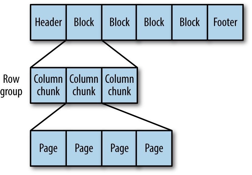
Figure 13-1. The internal structure of a Parquet file
Each page contains values from the same column, making a page a very good candidate for compression since the values are likely to be similar. The first level of compression is achieved through how the values are encoded. The simplest encoding is plain encoding, where values are written in full (e.g., an int32 is written using a 4-byte little-endian representation), but this doesn’t afford any compression in itself.
Parquet also uses more compact encodings, including delta encoding (the difference between values is stored), run-length encoding (sequences of identical values are encoded as a single value and the count), and dictionary encoding (a dictionary of values is built and itself encoded, then values are encoded as integers representing the indexes in the dictionary). In most cases, it also applies techniques such as bit packing to save space by storing several small values in a single byte.
When writing files, Parquet will choose an appropriate encoding automatically, based on the column type. For example, Boolean values will be written using a combination of runlength encoding and bit packing. Most types are encoded using dictionary encoding by default; however, a plain encoding will be used as a fallback if the dictionary becomes too large. The threshold size at which this happens is referred to as the _dictionary page size _and is the same as the page size by default (so the dictionary has to fit into one page if it is to be used). Note that the encoding that is actually used is stored in the file metadata to ensure that readers use the correct encoding.
In addition to the encoding, a second level of compression can be applied using a standard compression algorithm on the encoded page bytes. By default, no compression is applied, but Snappy, gzip, and LZO compressors are all supported.
For nested data, each page will also store the definition and repetition levels for all the values in the page. Since levels are small integers (the maximum is determined by the amount of nesting specified in the schema), they can be very efficiently encoded using a bit-packed run-length encoding.
Parquet Configuration
Parquet file properties are set at write time. The properties listed in Table 13-3 are appropriate if you are creating Parquet files from MapReduce (using the formats discussed in Parquet MapReduce), Crunch, Pig, or Hive.
Table 13-3. ParquetOutputFormat properties
| Property name Type | Default value | Description |
|---|---|---|
| parquet.block.size int | 134217728 (128 MB) |
The size in bytes of a block (row group). |
| parquet.page.size int | 1048576 (1 MB) |
The size in bytes of a page. |
| parquet.dictionary.page.size int | 1048576 (1 MB) |
The maximum allowed size in bytes of a dictionary before falling back to plain encoding for a page. |
| parquet.enable.dictionary boolean | true | Whether to use dictionary encoding. |
| parquet.compression String | UNCOMPRESSED The type of compression to use for Parquet files: UNCOMPRESSED, SNAPPY, GZIP, or LZO. Used instead of mapreduce.output.fileoutputformat.compress. |
Setting the block size is a trade-off between scanning efficiency and memory usage. Larger blocks are more efficient to scan through since they contain more rows, which improves sequential I/O (as there’s less overhead in setting up each column chunk). However, each block is buffered in memory for both reading and writing, which limits how large blocks can be. The default block size is 128 MB.
The Parquet file block size should be no larger than the HDFS block size for the file so that each Parquet block can be read from a single HDFS block (and therefore from a single datanode). It is common to set them to be the same, and indeed both defaults are for 128 MB block sizes.
A page is the smallest unit of storage in a Parquet file, so retrieving an arbitrary row (with a single column, for the sake of illustration) requires that the page containing the row be decompressed and decoded. Thus, for single-row lookups, it is more efficient to have smaller pages, so there are fewer values to read through before reaching the target value. However, smaller pages incur a higher storage and processing overhead, due to the extra metadata (offsets, dictionaries) resulting from more pages. The default page size is 1 MB.
Writing and Reading Parquet Files
Most of the time Parquet files are processed using higher-level tools like Pig, Hive, or Impala, but sometimes low-level sequential access may be required, which we cover in this section.
Parquet has a pluggable in-memory data model to facilitate integration of the Parquet file format with a wide range of tools and components. ReadSupport and WriteSupport are the integration points in Java, and implementations of these classes do the conversion between the objects used by the tool or component and the objects used to represent each Parquet type in the schema.
To demonstrate, we’ll use a simple in-memory model that comes bundled with Parquet in the parquet.example.data and parquet.example.data.simple packages. Then, in the
parquet.schema.MessageType:
MessageType schema = MessageTypeParser.parseMessageType(
“message Pair {\n” +
“ required binary left (UTF8);\n” +
“ required binary right (UTF8);\n” +
“}”);
Next, we need to create an instance of a Parquet message for each record to be written to the file. For the parquet.example.data package, a message is represented by an instance of Group, constructed using a GroupFactory:
GroupFactory groupFactory = new SimpleGroupFactory(schema);
Group group = groupFactory.newGroup()
.append(“left”, “L”)
.append(“right”, “R”);
Notice that the values in the message are UTF8 logical types, and Group provides a natural conversion from a Java String for us.
The following snippet of code shows how to create a Parquet file and write a message to it. The write() method would normally be called in a loop to write multiple messages to the file, but this only writes one here:
Configuration conf = new Configuration();
Path path = new Path(“data.parquet”);
GroupWriteSupport writeSupport = new GroupWriteSupport();
GroupWriteSupport.setSchema(schema, conf);
ParquetWriter
ParquetWriter.DEFAULTCOMPRESSION_CODEC_NAME,
ParquetWriter.DEFAULT_BLOCK_SIZE,
ParquetWriter.DEFAULT_PAGE_SIZE,
ParquetWriter.DEFAULT_PAGE_SIZE, / dictionary page size /
ParquetWriter.DEFAULT_IS_DICTIONARY_ENABLED,
ParquetWriter.DEFAULT_IS_VALIDATING_ENABLED,
ParquetProperties.WriterVersion.PARQUET_1_0, conf); writer.write(group); writer.close();
The ParquetWriter constructor needs to be provided with a WriteSupport instance, which defines how the message type is translated to Parquet’s types. In this case, we are using the Group message type, so GroupWriteSupport is used. Notice that the Parquet schema is set on the Configuration object by calling the setSchema() static method on GroupWriteSupport, and then the Configuration object is passed to ParquetWriter. This example also illustrates the Parquet file properties that may be set, corresponding to the ones listed in Table 13-3.
Reading a Parquet file is simpler than writing one, since the schema does not need to be specified as it is stored in the Parquet file. (It is, however, possible to set a _read schema to return a subset of the columns in the file, via projection.) Also, there are no file properties to be set since they are set at write time:
GroupReadSupport readSupport = new GroupReadSupport();
ParquetReader
ParquetReader has a read() method to read the next message. It returns null when the end of the file is reached:
Group result = reader.read(); assertNotNull(result); assertThat(result.getString(“left”, 0), is(“L”)); assertThat(result.getString(“right”, 0), is(“R”)); assertNull(reader.read());
Note that the 0 parameter passed to the getString() method specifies the index of the field to retrieve, since fields may have repeated values.
Avro, Protocol Buffers, and Thrift
Most applications will prefer to define models using a framework like Avro, Protocol
Buffers, or Thrift, and Parquet caters to all of these cases. Instead of ParquetWriter and
ParquetReader, use AvroParquetWriter, ProtoParquetWriter, or
ThriftParquetWriter, and the respective reader classes. These classes take care of translating between Avro, Protocol Buffers, or Thrift schemas and Parquet schemas (as well as performing the equivalent mapping between the framework types and Parquet types), which means you don’t need to deal with Parquet schemas directly.
Let’s repeat the previous example but using the Avro Generic API, just like we did in InMemory Serialization and Deserialization. The Avro schema is:
{
“type”: “record”,
“name”: “StringPair”,
“doc”: “A pair of strings.”,
“fields”: [
{“name”: “left”, “type”: “string”},
{“name”: “right”, “type”: “string”} ]
}
We create a schema instance and a generic record with:
Schema.Parser parser = new Schema.Parser();
Schema schema = parser.parse(getClass().getResourceAsStream(“StringPair.avsc”));
GenericRecord datum = new GenericData.Record(schema); datum.put(“left”, “L”); datum.put(“right”, “R”);
Then we can write a Parquet file:
Path path = new Path(“data.parquet”);
AvroParquetWriter
new AvroParquetWriter
AvroParquetWriter converts the Avro schema into a Parquet schema, and also translates each Avro GenericRecord instance into the corresponding Parquet types to write to the Parquet file. The file is a regular Parquet file — it is identical to the one written in the previous section using ParquetWriter with GroupWriteSupport, except for an extra piece of metadata to store the Avro schema. We can see this by inspecting the file’s metadata using Parquet’s command-line tools:89]
% parquet-tools meta data.parquet
…
extra: avro.schema = {“type”:”record”,”name”:”StringPair”, … …
Similarly, to see the Parquet schema that was generated from the Avro schema, we can use the following:
% parquet-tools schema data.parquet message StringPair { required binary left (UTF8); required binary right (UTF8);
}
To read the Parquet file back, we use an AvroParquetReader and get back Avro GenericRecord objects:
AvroParquetReader
Projection and read schemas
It’s often the case that you only need to read a few columns in the file, and indeed this is the raison d’être of a columnar format like Parquet: to save time and I/O. You can use a projection schema to select the columns to read. For example, the following schema will read only the right field of a StringPair:
{
“type”: “record”,
“name”: “StringPair”,
“doc”: “The right field of a pair of strings.”, “fields”: [
{“name”: “right”, “type”: “string”}
] }
In order to use a projection schema, set it on the configuration using the setRequestedProjection() static convenience method on AvroReadSupport:
Schema projectionSchema = parser.parse(
getClass().getResourceAsStream(“ProjectedStringPair.avsc”));
Configuration conf = new Configuration();
AvroReadSupport.setRequestedProjection(conf, projectionSchema);
Then pass the configuration into the constructor for AvroParquetReader:
AvroParquetReader
new AvroParquetReader
Both the Protocol Buffers and Thrift implementations support projection in a similar manner. In addition, the Avro implementation allows you to specify a reader’s schema by calling setReadSchema() on AvroReadSupport. This schema is used to resolve Avro records according to the rules listed in Table 12-4.
The reason that Avro has both a projection schema and a reader’s schema is that the projection must be a subset of the schema used to write the Parquet file, so it cannot be used to evolve a schema by adding new fields.
The two schemas serve different purposes, and you can use both together. The projection schema is used to filter the columns to read from the Parquet file. Although it is expressed as an Avro schema, it can be viewed simply as a list of Parquet columns to read back. The reader’s schema, on the other hand, is used only to resolve Avro records. It is never translated to a Parquet schema, since it has no bearing on which columns are read from the
Parquet file. For example, if we added a description field to our Avro schema (like in Schema Resolution) and used it as the Avro reader’s schema, then the records would contain the default value of the field, even though the Parquet file has no such field.
Parquet MapReduce
Parquet comes with a selection of MapReduce input and output formats for reading and writing Parquet files from MapReduce jobs, including ones for working with Avro, Protocol Buffers, and Thrift schemas and data.
The program in Example 13-1 is a map-only job that reads text files and writes Parquet files where each record is the line’s offset in the file (represented by an int64 — converted from a long in Avro) and the line itself (a string). It uses the Avro Generic API for its in-memory data model.
Example 13-1. MapReduce program to convert text files to Parquet files using AvroParquetOutputFormat
public class TextToParquetWithAvro extends Configured implements Tool {
private static final Schema SCHEMA = new Schema.Parser().parse(
“{\n” +
“ \”type\”: \”record\”,\n” +
“ \”name\”: \”Line\”,\n” +
“ \”fields\”: [\n” +
“ {\”name\”: \”offset\”, \”type\”: \”long\”},\n” + “ {\”name\”: \”line\”, \”type\”: \”string\”}\n” +
“ ]\n” + “}”);
public static class TextToParquetMapper
extends Mapper
@Override
protected void map(LongWritable key, Text value, Context context) throws IOException, InterruptedException { record.put(“offset”, key.get()); record.put(“line”, value.toString()); context.write(null, record);
}
}
@Override
public int run(String[] args) throws Exception { if (args.length != 2) {
System.err.printf(“Usage: %s [generic options]
Chapter 14. Flume
Hadoop is built for processing very large datasets. Often it is assumed that the data is already in HDFS, or can be copied there in bulk. However, there are many systems that don’t meet this assumption. They produce streams of data that we would like to aggregate, store, and analyze using Hadoop — and these are the systems that Apache Flume is an ideal fit for.
Flume is designed for high-volume ingestion into Hadoop of event-based data. The canonical example is using Flume to collect logfiles from a bank of web servers, then moving the log events from those files into new aggregated files in HDFS for processing. The usual destination (or sink in Flume parlance) is HDFS. However, Flume is flexible enough to write to other systems, like HBase or Solr.
To use Flume, we need to run a Flume agent, which is a long-lived Java process that runs sources and sinks, connected by channels. A source in Flume produces events and delivers them to the channel, which stores the events until they are forwarded to the sink. You can think of the source-channel-sink combination as a basic Flume building block.
A Flume installation is made up of a collection of connected agents running in a distributed topology. Agents on the edge of the system (co-located on web server machines, for example) collect data and forward it to agents that are responsible for aggregating and then storing the data in its final destination. Agents are configured to run a collection of particular sources and sinks, so using Flume is mainly a configuration exercise in wiring the pieces together. In this chapter, we’ll see how to build Flume topologies for data ingestion that you can use as a part of your own Hadoop pipeline.
Installing Flume
Download a stable release of the Flume binary distribution from the download page, and unpack the tarball in a suitable location:
% tar xzf apache-flume-x.y.z-bin.tar.gz
It’s useful to put the Flume binary on your path:
% export FLUMEHOME=~/sw/apache-flume-_x.y.z-bin
% export PATH=$PATH:$FLUME_HOME/bin
A Flume agent can then be started with the flume-ng command, as we’ll see next.
An Example
To show how Flume works, let’s start with a setup that:
1. Watches a local directory for new text files
2. Sends each line of each file to the console as files are added
We’ll add the files by hand, but it’s easy to imagine a process like a web server creating new files that we want to continuously ingest with Flume. Also, in a real system, rather than just logging the file contents we would write the contents to HDFS for subsequent processing — we’ll see how to do that later in the chapter.
In this example, the Flume agent runs a single source-channel-sink, configured using a Java properties file. The configuration controls the types of sources, sinks, and channels that are used, as well as how they are connected together. For this example, we’ll use the configuration in Example 14-1.
Example 14-1. Flume configuration using a spooling directory source and a logger sink
agent1.sources = source1 agent1.sinks = sink1 agent1.channels = channel1
agent1.sources.source1.channels = channel1 agent1.sinks.sink1.channel = channel1
agent1.sources.source1.type = spooldir agent1.sources.source1.spoolDir = /tmp/spooldir agent1.sinks.sink1.type = logger agent1.channels.channel1.type = file
Property names form a hierarchy with the agent name at the top level. In this example, we have a single agent, called agent1. The names for the different components in an agent are defined at the next level, so for example agent1.sources lists the names of the sources that should be run in agent1 (here it is a single source, source1). Similarly, agent1 has a sink (sink1) and a channel (channel1).
The properties for each component are defined at the next level of the hierarchy. The configuration properties that are available for a component depend on the type of the component. In this case, agent1.sources.source1.type is set to spooldir, which is a spooling directory source that monitors a spooling directory for new files. The spooling directory source defines a spoolDir property, so for source1 the full key is agent1.sources.source1.spoolDir. The source’s channels are set with agent1.sources.source1.channels.
The sink is a logger sink for logging events to the console. It too must be connected to the channel (with the agent1.sinks.sink1.channel property).90] The channel is a file channel, which means that events in the channel are persisted to disk for durability. The system is illustrated in Figure 14-1.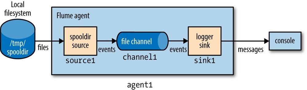
Figure 14-1. Flume agent with a spooling directory source and a logger sink connected by a file channel
Before running the example, we need to create the spooling directory on the local filesystem:
% mkdir /tmp/spooldir
Then we can start the Flume agent using the flume-ng command:
% flume-ng agent \
—conf-file spool-to-logger.properties \
—name agent1 \
—conf $FLUME_HOME/conf \
-Dflume.root.logger=INFO,console
The Flume properties file from Example 14-1 is specified with the —conf-file flag. The agent name must also be passed in with —name (since a Flume properties file can define several agents, we have to say which one to run). The —conf flag tells Flume where to find its general configuration, such as environment settings.
In a new terminal, create a file in the spooling directory. The spooling directory source expects files to be immutable. To prevent partially written files from being read by the source, we write the full contents to a hidden file. Then, we do an atomic rename so the source can read it:91]
% echo “Hello Flume” > /tmp/spooldir/.file1.txt
% mv /tmp/spooldir/.file1.txt /tmp/spooldir/file1.txt
Back in the agent’s terminal, we see that Flume has detected and processed the file:
Preparing to move file /tmp/spooldir/file1.txt to
/tmp/spooldir/file1.txt.COMPLETED
Event: { headers:{} body: 48 65 6C 6C 6F 20 46 6C 75 6D 65 Hello Flume }
The spooling directory source ingests the file by splitting it into lines and creating a Flume event for each line. Events have optional headers and a binary body, which is the UTF-8 representation of the line of text. The body is logged by the logger sink in both hexadecimal and string form. The file we placed in the spooling directory was only one line long, so only one event was logged in this case. We also see that the file was renamed to file1.txt.COMPLETED by the source, which indicates that Flume has completed processing it and won’t process it again.
Transactions and Reliability
Flume uses separate transactions to guarantee delivery from the source to the channel and from the channel to the sink. In the example in the previous section, the spooling directory source creates an event for each line in the file. The source will only mark the file as completed once the transactions encapsulating the delivery of the events to the channel have been successfully committed.
Similarly, a transaction is used for the delivery of the events from the channel to the sink. If for some unlikely reason the events could not be logged, the transaction would be rolled back and the events would remain in the channel for later redelivery.
The channel we are using is a file channel, which has the property of being durable: once an event has been written to the channel, it will not be lost, even if the agent restarts. (Flume also provides a memory channel that does not have this property, since events are stored in memory. With this channel, events are lost if the agent restarts. Depending on the application, this might be acceptable. The trade-off is that the memory channel has higher throughput than the file channel.)
The overall effect is that every event produced by the source will reach the sink. The major caveat here is that every event will reach the sink at least once — that is, duplicates are possible. Duplicates can be produced in sources or sinks: for example, after an agent restart, the spooling directory source will redeliver events for an uncompleted file, even if some or all of them had been committed to the channel before the restart. After a restart, the logger sink will re-log any event that was logged but not committed (which could happen if the agent was shut down between these two operations).
At-least-once semantics might seem like a limitation, but in practice it is an acceptable performance trade-off. The stronger semantics of exactly once require a two-phase commit protocol, which is expensive. This choice is what differentiates Flume (at-least-once semantics) as a high-volume parallel event ingest system from more traditional enterprise messaging systems (exactly-once semantics). With at-least-once semantics, duplicate events can be removed further down the processing pipeline. Usually this takes the form of an application-specific deduplication job written in MapReduce or Hive.
Batching
For efficiency, Flume tries to process events in batches for each transaction, where possible, rather than one by one. Batching helps file channel performance in particular, since every transaction results in a local disk write and fsync call.
The batch size used is determined by the component in question, and is configurable in many cases. For example, the spooling directory source will read files in batches of 100 lines. (This can be changed by setting the batchSize property.) Similarly, the Avro sink (discussed in Distribution: Agent Tiers) will try to read 100 events from the channel before sending them over RPC, although it won’t block if fewer are available.
The HDFS Sink
The point of Flume is to deliver large amounts of data into a Hadoop data store, so let’s look at how to configure a Flume agent to deliver events to an HDFS sink. The configuration in Example 14-2 updates the previous example to use an HDFS sink. The only two settings that are required are the sink’s type (hdfs) and hdfs.path, which specifies the directory where files will be placed (if, like here, the filesystem is not specified in the path, it’s determined in the usual way from Hadoop’s fs.defaultFS property). We’ve also specified a meaningful file prefix and suffix, and instructed Flume to write events to the files in text format.
Example 14-2. Flume configuration using a spooling directory source and an HDFS sink
agent1.sources = source1 agent1.sinks = sink1 agent1.channels = channel1
agent1.sources.source1.channels = channel1 agent1.sinks.sink1.channel = channel1
agent1.sources.source1.type = spooldir agent1.sources.source1.spoolDir = /tmp/spooldir
agent1.sinks.sink1.type = hdfs agent1.sinks.sink1.hdfs.path = /tmp/flume agent1.sinks.sink1.hdfs.filePrefix = events agent1.sinks.sink1.hdfs.fileSuffix = .log agent1.sinks.sink1.hdfs.inUsePrefix = _ agent1.sinks.sink1.hdfs.fileType = DataStream agent1.channels.channel1.type = file
Restart the agent to use the spool-to-hdfs.properties configuration, and create a new file in the spooling directory:
% echo -e “Hello\nAgain” > /tmp/spooldir/.file2.txt
% mv /tmp/spooldir/.file2.txt /tmp/spooldir/file2.txt
Events will now be delivered to the HDFS sink and written to a file. Files in the process of being written to have a .tmp in-use suffix added to their name to indicate that they are not yet complete. In this example, we have also set hdfs.inUsePrefix to be (underscore; by default it is empty), which causes files in the process of being written to have that prefix added to their names. This is useful since MapReduce will ignore files that have a prefix. So, a typical temporary filename would be _events.1399295780136.log.tmp; the number is a timestamp generated by the HDFS sink.
A file is kept open by the HDFS sink until it has either been open for a given time (default
30 seconds, controlled by the hdfs.rollInterval property), has reached a given size (default 1,024 bytes, set by hdfs.rollSize), or has had a given number of events written to it (default 10, set by hdfs.rollCount). If any of these criteria are met, the file is closed and its in-use prefix and suffix are removed. New events are written to a new file (which will have an in-use prefix and suffix until it is rolled).
After 30 seconds, we can be sure that the file has been rolled and we can take a look at its contents:
% hadoop fs -cat /tmp/flume/events.1399295780136.log
Hello
Again
The HDFS sink writes files as the user who is running the Flume agent, unless the hdfs.proxyUser property is set, in which case files will be written as that user.
Partitioning and Interceptors
Large datasets are often organized into partitions, so that processing can be restricted to particular partitions if only a subset of the data is being queried. For Flume event data, it’s very common to partition by time. A process can be run periodically that transforms completed partitions (to remove duplicate events, for example).
It’s easy to change the example to store data in partitions by setting hdfs.path to include subdirectories that use time format escape sequences: agent1.sinks.sink1.hdfs.path = /tmp/flume/year=%Y/month=%m/day=%d
Here we have chosen to have day-sized partitions, but other levels of granularity are possible, as are other directory layout schemes. (If you are using Hive, see Partitions and Buckets for how Hive lays out partitions on disk.) The full list of format escape sequences is provided in the documentation for the HDFS sink in the Flume User Guide.
The partition that a Flume event is written to is determined by the timestamp header on the event. Events don’t have this header by default, but it can be added using a Flume interceptor. Interceptors are components that can modify or drop events in the flow; they are attached to sources, and are run on events before the events have been placed in a channel.92] The following extra configuration lines add a timestamp interceptor to source1, which adds a timestamp header to every event produced by the source:
agent1.sources.source1.interceptors = interceptor1 agent1.sources.source1.interceptors.interceptor1.type = timestamp
Using the timestamp interceptor ensures that the timestamps closely reflect the times at which the events were created. For some applications, using a timestamp for when the event was written to HDFS might be sufficient — although, be aware that when there are multiple tiers of Flume agents there can be a significant difference between creation time and write time, especially in the event of agent downtime (see Distribution: Agent Tiers). For these cases, the HDFS sink has a setting, hdfs.useLocalTimeStamp, that will use a timestamp generated by the Flume agent running the HDFS sink.
File Formats
It’s normally a good idea to use a binary format for storing your data in, since the resulting files are smaller than they would be if you used text. For the HDFS sink, the file format used is controlled using hdfs.fileType and a combination of a few other properties.
If unspecified, hdfs.fileType defaults to SequenceFile, which will write events to a sequence file with LongWritable keys that contain the event timestamp (or the current time if the timestamp header is not present) and BytesWritable values that contain the event body. It’s possible to use Text Writable values in the sequence file instead of BytesWritable by setting hdfs.writeFormat to Text.
The configuration is a little different for Avro files. The hdfs.fileType property is set to DataStream, just like for plain text. Additionally, serializer (note the lack of an hdfs. prefix) must be set to avro_event. To enable compression, set the
serializer.compressionCodec property. Here is an example of an HDFS sink configured to write Snappy-compressed Avro files:
agent1.sinks.sink1.type = hdfs agent1.sinks.sink1.hdfs.path = /tmp/flume agent1.sinks.sink1.hdfs.filePrefix = events agent1.sinks.sink1.hdfs.fileSuffix = .avro agent1.sinks.sink1.hdfs.fileType = DataStream agent1.sinks.sink1.serializer = avro_event agent1.sinks.sink1.serializer.compressionCodec = snappy
An event is represented as an Avro record with two fields: headers, an Avro map with string values, and body, an Avro bytes field.
If you want to use a custom Avro schema, there are a couple of options. If you have Avro in-memory objects that you want to send to Flume, then the Log4jAppender is appropriate. It allows you to log an Avro Generic, Specific, or Reflect object using a log4j Logger and send it to an Avro source running in a Flume agent (see Distribution: Agent Tiers). In this case, the serializer property for the HDFS sink should be set to org.apache.flume.sink.hdfs.AvroEventSerializer$Builder, and the Avro schema set in the header (see the class documentation).
Alternatively, if the events are not originally derived from Avro objects, you can write a custom serializer to convert a Flume event into an Avro object with a custom schema. The helper class AbstractAvroEventSerializer in the org.apache.flume.serialization package is a good starting point.
Fan Out
Fan out is the term for delivering events from one source to multiple channels, so they reach multiple sinks. For example, the configuration in Example 14-3 delivers events to both an HDFS sink (sink1a via channel1a) and a logger sink (sink1b via channel1b).
Example 14-3. Flume configuration using a spooling directory source, fanning out to an HDFS sink and a logger sink
agent1.sources = source1 agent1.sinks = sink1a sink1b agent1.channels = channel1a channel1b
agent1.sources.source1.channels = channel1a channel1b agent1.sinks.sink1a.channel = channel1a agent1.sinks.sink1b.channel = channel1b
agent1.sources.source1.type = spooldir agent1.sources.source1.spoolDir = /tmp/spooldir
agent1.sinks.sink1a.type = hdfs agent1.sinks.sink1a.hdfs.path = /tmp/flume agent1.sinks.sink1a.hdfs.filePrefix = events agent1.sinks.sink1a.hdfs.fileSuffix = .log agent1.sinks.sink1a.hdfs.fileType = DataStream agent1.sinks.sink1b.type = logger
agent1.channels.channel1a.type = file agent1.channels.channel1b.type = memory
The key change here is that the source is configured to deliver to multiple channels by setting agent1.sources.source1.channels to a space-separated list of channel names, channel1a and channel1b. This time, the channel feeding the logger sink (channel1b) is a memory channel, since we are logging events for debugging purposes and don’t mind losing events on agent restart. Also, each channel is configured to feed one sink, just like in the previous examples. The flow is illustrated in Figure 14-2.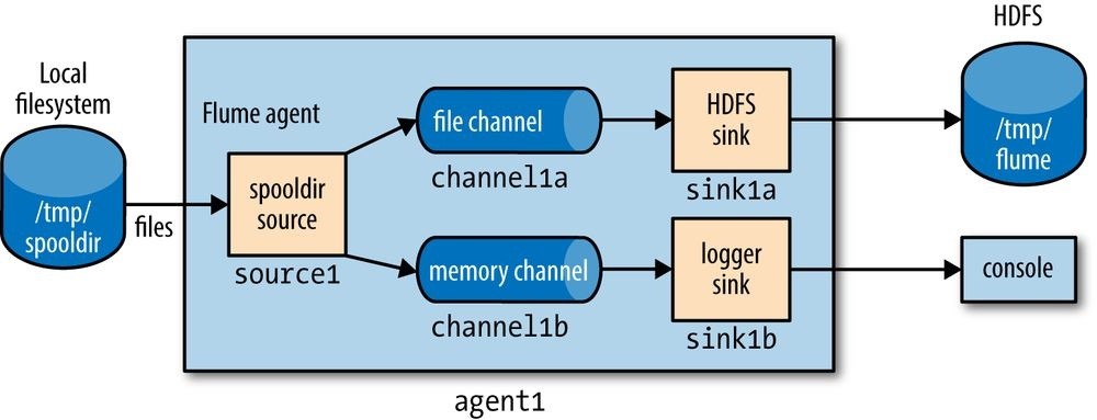
Figure 14-2. Flume agent with a spooling directory source and fanning out to an HDFS sink and a logger sink
Delivery Guarantees
Flume uses a separate transaction to deliver each batch of events from the spooling directory source to each channel. In this example, one transaction will be used to deliver to the channel feeding the HDFS sink, and then another transaction will be used to deliver
the same batch of events to the channel for the logger sink. If either of these transactions fails (if a channel is full, for example), then the events will not be removed from the source, and will be retried later.
In this case, since we don’t mind if some events are not delivered to the logger sink, we can designate its channel as an optional channel, so that if the transaction associated with it fails, this will not cause events to be left in the source and tried again later. (Note that if the agent fails before both channel transactions have committed, then the affected events will be redelivered after the agent restarts — this is true even if the uncommitted channels are marked as optional.) To do this, we set the selector.optional property on the source, passing it a space-separated list of channels: agent1.sources.source1.selector.optional = channel1b
NEAR-REAL-TIME INDEXING
Indexing events for search is a good example of where fan out is used in practice. A single source of events is sent to both an HDFS sink (this is the main repository of events, so a required channel is used) and a Solr (or Elasticsearch) sink, to build a search index (using an optional channel).
The MorphlineSolrSink extracts fields from Flume events and transforms them into a Solr document (using a Morphline configuration file), which is then loaded into a live Solr search server. The process is called _near real time _since ingested data appears in search results in a matter of seconds.
Replicating and Multiplexing Selectors
In normal fan-out flow, events are replicated to all channels — but sometimes more selective behavior might be desirable, so that some events are sent to one channel and others to another. This can be achieved by setting a multiplexing selector on the source, and defining routing rules that map particular event header values to channels. See the Flume User Guide for configuration details.
Distribution: Agent Tiers
How do we scale a set of Flume agents? If there is one agent running on every node producing raw data, then with the setup described so far, at any particular time each file being written to HDFS will consist entirely of the events from one node. It would be better if we could aggregate the events from a group of nodes in a single file, since this would result in fewer, larger files (with the concomitant reduction in pressure on HDFS, and more efficient processing in MapReduce; see Small files and CombineFileInputFormat). Also, if needed, files can be rolled more often since they are being fed by a larger number of nodes, leading to a reduction between the time when an event is created and when it’s available for analysis.
Aggregating Flume events is achieved by having tiers of Flume agents. The first tier collects events from the original sources (such as web servers) and sends them to a smaller set of agents in the second tier, which aggregate events from the first tier before writing them to HDFS (see Figure 14-3). Further tiers may be warranted for very large numbers of source nodes.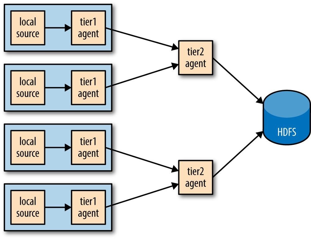
Figure 14-3. Using a second agent tier to aggregate Flume events from the first tier
Tiers are constructed by using a special sink that sends events over the network, and a corresponding source that receives events. The Avro sink sends events over Avro RPC to an Avro source running in another Flume agent. There is also a Thrift sink that does the same thing using Thrift RPC, and is paired with a Thrift source.93]
WARNING
Don’t be confused by the naming: Avro sinks and sources do not provide the ability to write (or read) Avro files. They are used only to distribute events between agent tiers, and to do so they use Avro RPC to communicate (hence the name). If you need to write events to Avro files, use the HDFS sink, described in File Formats.
Example 14-4 shows a two-tier Flume configuration. Two agents are defined in the file, named agent1 and agent2. An agent of type agent1 runs in the first tier, and has a spooldir source and an Avro sink connected by a file channel. The agent2 agent runs in the second tier, and has an Avro source that listens on the port that agent1’s Avro sink sends events to. The sink for agent2 uses the same HDFS sink configuration from Example 14-2.
Notice that since there are two file channels running on the same machine, they are configured to point to different data and checkpoint directories (they are in the user’s home directory by default). This way, they don’t try to write their files on top of one another.
Example 14-4. A two-tier Flume configuration using a spooling directory source and an HDFS sink
# First-tier agent
agent1.sources = source1 agent1.sinks = sink1 agent1.channels = channel1
agent1.sources.source1.channels = channel1 agent1.sinks.sink1.channel = channel1
agent1.sources.source1.type = spooldir agent1.sources.source1.spoolDir = /tmp/spooldir
agent1.sinks.sink1.type = avro agent1.sinks.sink1.hostname = localhost agent1.sinks.sink1.port = 10000
agent1.channels.channel1.type = file agent1.channels.channel1.checkpointDir=/tmp/agent1/file-channel/checkpoint agent1.channels.channel1.dataDirs=/tmp/agent1/file-channel/data
# Second-tier agent
agent2.sources = source2 agent2.sinks = sink2 agent2.channels = channel2
agent2.sources.source2.channels = channel2 agent2.sinks.sink2.channel = channel2
agent2.sources.source2.type = avro agent2.sources.source2.bind = localhost agent2.sources.source2.port = 10000
agent2.sinks.sink2.type = hdfs agent2.sinks.sink2.hdfs.path = /tmp/flume agent2.sinks.sink2.hdfs.filePrefix = events agent2.sinks.sink2.hdfs.fileSuffix = .log agent2.sinks.sink2.hdfs.fileType = DataStream
agent2.channels.channel2.type = file agent2.channels.channel2.checkpointDir=/tmp/agent2/file-channel/checkpoint agent2.channels.channel2.dataDirs=/tmp/agent2/file-channel/data The system is illustrated in Figure 14-4.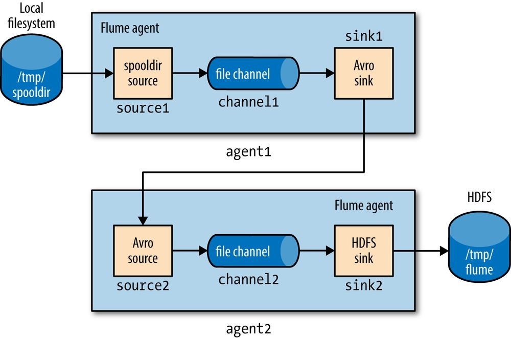
Figure 14-4. Two Flume agents connected by an Avro sink-source pair
Each agent is run independently, using the same —conf-file parameter but different agent —name parameters:
% flume-ng agent —conf-file spool-to-hdfs-tiered.properties —name agent1… and:
% flume-ng agent —conf-file spool-to-hdfs-tiered.properties —name agent2…
Delivery Guarantees
Flume uses transactions to ensure that each batch of events is reliably delivered from a source to a channel, and from a channel to a sink. In the context of the Avro sink-source connection, transactions ensure that events are reliably delivered from one agent to the next.
The operation to read a batch of events from the file channel in agent1 by the Avro sink will be wrapped in a transaction. The transaction will only be committed once the Avro sink has received the (synchronous) confirmation that the write to the Avro source’s RPC endpoint was successful. This confirmation will only be sent once agent2’s transaction wrapping the operation to write the batch of events to its file channel has been successfully committed. Thus, the Avro sink-source pair guarantees that an event is delivered from one Flume agent’s channel to another Flume agent’s channel (at least once).
If either agent is not running, then clearly events cannot be delivered to HDFS. For example, if agent1 stops running, then files will accumulate in the spooling directory, to be processed once agent1 starts up again. Also, any events in an agent’s own file channel at the point the agent stopped running will be available on restart, due to the durability guarantee that file channel provides.
If agent2 stops running, then events will be stored in agent1’s file channel until agent2 starts again. Note, however, that channels necessarily have a limited capacity; if agent1’s channel fills up while agent2 is not running, then any new events will be lost. By default, a file channel will not recover more than one million events (this can be overridden by its capacity property), and it will stop accepting events if the free disk space for its checkpoint directory falls below 500 MB (controlled by the minimumRequiredSpace property).
Both these scenarios assume that the agent will eventually recover, but that is not always the case (if the hardware it is running on fails, for example). If agent1 doesn’t recover, then the loss is limited to the events in its file channel that had not been delivered to agent2 before agent1 shut down. In the architecture described here, there are multiple first-tier agents like agent1, so other nodes in the tier can take over the function of the failed node. For example, if the nodes are running load-balanced web servers, then other nodes will absorb the failed web server’s traffic, and they will generate new Flume events that are delivered to agent2. Thus, no new events are lost.
An unrecoverable agent2 failure is more serious, however. Any events in the channels of upstream first-tier agents (agent1 instances) will be lost, and all new events generated by these agents will not be delivered either. The solution to this problem is for agent1 to have multiple redundant Avro sinks, arranged in a sink group, so that if the destination agent2 Avro endpoint is unavailable, it can try another sink from the group. We’ll see how to do this in the next section.
Sink Groups
A sink group allows multiple sinks to be treated as one, for failover or load-balancing purposes (see Figure 14-5). If a second-tier agent is unavailable, then events will be delivered to another second-tier agent and on to HDFS without disruption.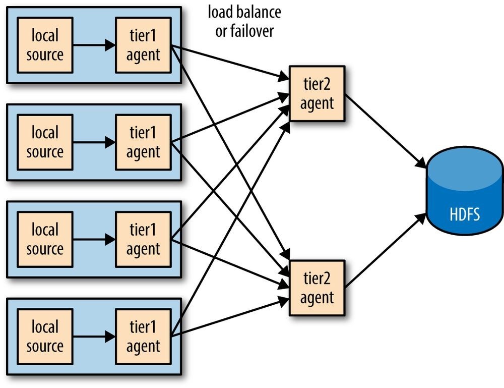
Figure 14-5. Using multiple sinks for load balancing or failover
To configure a sink group, the agent’s sinkgroups property is set to define the sink group’s name; then the sink group lists the sinks in the group, and also the type of the sink processor, which sets the policy for choosing a sink. Example 14-5 shows the configuration for load balancing between two Avro endpoints.
Example 14-5. A Flume configuration for load balancing between two Avro endpoints using a sink group
agent1.sources = source1 agent1.sinks = sink1a sink1b agent1.sinkgroups = sinkgroup1 agent1.channels = channel1
agent1.sources.source1.channels = channel1 agent1.sinks.sink1a.channel = channel1 agent1.sinks.sink1b.channel = channel1
agent1.sinkgroups.sinkgroup1.sinks = sink1a sink1b agent1.sinkgroups.sinkgroup1.processor.type = load_balance agent1.sinkgroups.sinkgroup1.processor.backoff = true agent1.sources.source1.type = spooldir agent1.sources.source1.spoolDir = /tmp/spooldir
agent1.sinks.sink1a.type = avro agent1.sinks.sink1a.hostname = localhost agent1.sinks.sink1a.port = 10000
agent1.sinks.sink1b.type = avro agent1.sinks.sink1b.hostname = localhost agent1.sinks.sink1b.port = 10001 agent1.channels.channel1.type = file
There are two Avro sinks defined, sink1a and sink1b, which differ only in the Avro endpoint they are connected to (since we are running all the examples on localhost, it is the port that is different; for a distributed install, the hosts would differ and the ports would be the same). We also define sinkgroup1, and set its sinks to sink1a and sink1b.
The processor type is set to load_balance, which attempts to distribute the event flow over both sinks in the group, using a round-robin selection mechanism (you can change this using the processor.selector property). If a sink is unavailable, then the next sink is tried; if they are all unavailable, the event is not removed from the channel, just like in the single sink case. By default, sink unavailability is not remembered by the sink processor, so failing sinks are retried for every batch of events being delivered. This can be inefficient, so we have set the processor.backoff property to change the behavior so that failing sinks are blacklisted for an exponentially increasing timeout period (up to a maximum period of 30 seconds, controlled by processor.selector.maxTimeOut).
NOTE
There is another type of processor, failover, that instead of load balancing events across sinks uses a preferred sink if it is available, and fails over to another sink in the case that the preferred sink is down. The failover sink processor maintains a priority order for sinks in the group, and attempts delivery in order of priority. If the sink with the highest priority is unavailable the one with the next highest priority is tried, and so on. Failed sinks are blacklisted for an increasing timeout period (up to a maximum period of 30 seconds, controlled by processor.maxpenalty).
The configuration for one of the second-tier agents, agent2a, is shown in Example 14-6. Example 14-6. Flume configuration for second-tier agent in a load balancing scenario
agent2a.sources = source2a agent2a.sinks = sink2a agent2a.channels = channel2a
agent2a.sources.source2a.channels = channel2a agent2a.sinks.sink2a.channel = channel2a
agent2a.sources.source2a.type = avro agent2a.sources.source2a.bind = localhost agent2a.sources.source2a.port = 10000
agent2a.sinks.sink2a.type = hdfs agent2a.sinks.sink2a.hdfs.path = /tmp/flume agent2a.sinks.sink2a.hdfs.filePrefix = events-a agent2a.sinks.sink2a.hdfs.fileSuffix = .log agent2a.sinks.sink2a.hdfs.fileType = DataStream agent2a.channels.channel2a.type = file
The configuration for agent2b is the same, except for the Avro source port (since we are running the examples on localhost) and the file prefix for the files created by the HDFS sink. The file prefix is used to ensure that HDFS files created by second-tier agents at the same time don’t collide.
In the more usual case of agents running on different machines, the hostname can be used to make the filename unique by configuring a host interceptor (see Table 14-1) and including the %{host} escape sequence in the file path, or prefix: agent2.sinks.sink2.hdfs.filePrefix = events-%{host}
A diagram of the whole system is shown in Figure 14-6.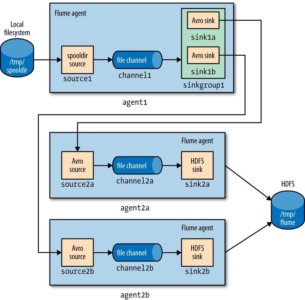
Figure 14-6. Load balancing between two agents
Integrating Flume with Applications
An Avro source is an RPC endpoint that accepts Flume events, making it possible to write an RPC client to send events to the endpoint, which can be embedded in any application that wants to introduce events into Flume.
The Flume SDK is a module that provides a Java RpcClient class for sending Event objects to an Avro endpoint (an Avro source running in a Flume agent, usually in another tier). Clients can be configured to fail over or load balance between endpoints, and Thrift endpoints (Thrift sources) are supported too.
The Flume embedded agent offers similar functionality: it is a cut-down Flume agent that runs in a Java application. It has a single special source that your application sends Flume Event objects to by calling a method on the EmbeddedAgent object; the only sinks that are supported are Avro sinks, but it can be configured with multiple sinks for failover or load balancing.
Both the SDK and the embedded agent are described in more detail in the Flume Developer Guide.
Component Catalog
We’ve only used a handful of Flume components in this chapter. Flume comes with many more, which are briefly described in Table 14-1. Refer to the Flume User Guide for further information on how to configure and use them.
_Table 14-1. Flume components _Category Component Description
| Source | Avro | Listens on a port for events sent over Avro RPC by an Avro sink or the Flume SDK. |
|---|---|---|
| Exec | Runs a Unix command (e.g., tail -F/path/to/file) and converts lines read from standard output into events. Note that this source cannot guarantee delivery of events to the channel; see the spooling directory source or the Flume SDK for better alternatives. | |
| HTTP | Listens on a port and converts HTTP requests into events using a pluggable handler (e.g., a JSON handler or binary blob handler). | |
| JMS | Reads messages from a JMS queue or topic and converts them into events. | |
| Netcat | Listens on a port and converts each line of text into an event. | |
| Sequence generator | Generates events from an incrementing counter. Useful for testing. | |
| Spooling directory | Reads lines from files placed in a spooling directory and converts them into events. | |
| Syslog | Reads lines from syslog and converts them into events. | |
| Thrift | Listens on a port for events sent over Thrift RPC by a Thrift sink or the Flume SDK. | |
| Connects to Twitter’s streaming API (1% of the firehose) and converts tweets into events. | ||
| Sink | Avro | Sends events over Avro RPC to an Avro source. |
| Elasticsearch | Writes events to an Elasticsearch cluster using the Logstash format. | |
| File roll | Writes events to the local filesystem. | |
| HBase | Writes events to HBase using a choice of serializer. | |
| HDFS | Writes events to HDFS in text, sequence file, Avro, or a custom format. | |
| IRC | Sends events to an IRC channel. | |
| Logger | Logs events at INFO level using SLF4J. Useful for testing. | |
| Morphline (Solr) |
Runs events through an in-process chain of Morphline commands. Typically used to load data into Solr. | |
| Null | Discards all events. | |
| Thrift | Sends events over Thrift RPC to a Thrift source. | |
| Channel | File | Stores events in a transaction log stored on the local filesystem. |
| JDBC | Stores events in a database (embedded Derby). |
Memory Stores events in an in-memory queue.
| Interceptor | Host | Sets a host header containing the agent’s hostname or IP address on all events. |
|---|---|---|
| Morphline | Filters events through a Morphline configuration file. Useful for conditionally dropping events or adding headers based on pattern matching or content extraction. | |
| Regex extractor |
Sets headers extracted from the event body as text using a specified regular expression. | |
| Regex filtering |
Includes or excludes events by matching the event body as text against a specified regular expression. | |
| Static | Sets a fixed header and value on all events. | |
| Timestamp | Sets a timestamp header containing the time in milliseconds at which the agent processes the event. | |
| UUID | Sets an id header containing a universally unique identifier on all events. Useful for later deduplication. |
Further Reading
This chapter has given a short overview of Flume. For more detail, see Using Flume by Hari Shreedharan (O’Reilly, 2014). There is also a lot of practical information about designing ingest pipelines (and building Hadoop applications in general) in Hadoop Application Architectures by Mark Grover, Ted Malaska, Jonathan Seidman, and Gwen Shapira (O’Reilly, 2014).
[90] Note that a source has a channels property (plural) but a sink has a channel property (singular). This is because a source can feed more than one channel (see Fan Out), but a sink can only be fed by one channel. It’s also possible for a channel to feed multiple sinks. This is covered in Sink Groups.
[91] For a logfile that is continually appended to, you would periodically roll the logfile and move the old file to the spooling directory for Flume to read it.
[92] Table 14-1 describes the interceptors that Flume provides.
[93] The Avro sink-source pair is older than the Thrift equivalent, and (at the time of writing) has some features that the Thrift one doesn’t provide, such as encryption.
Chapter 15. Sqoop
Aaron Kimball
A great strength of the Hadoop platform is its ability to work with data in several different forms. HDFS can reliably store logs and other data from a plethora of sources, and MapReduce programs can parse diverse ad hoc data formats, extracting relevant information and combining multiple datasets into powerful results.
But to interact with data in storage repositories outside of HDFS, MapReduce programs need to use external APIs. Often, valuable data in an organization is stored in structured data stores such as relational database management systems (RDBMSs). Apache Sqoop is an open source tool that allows users to extract data from a structured data store into Hadoop for further processing. This processing can be done with MapReduce programs or other higher-level tools such as Hive. (It’s even possible to use Sqoop to move data from a database into HBase.) When the final results of an analytic pipeline are available, Sqoop can export these results back to the data store for consumption by other clients.
In this chapter, we’ll take a look at how Sqoop works and how you can use it in your data processing pipeline.
Getting Sqoop
Sqoop is available in a few places. The primary home of the project is the Apache Software Foundation. This repository contains all the Sqoop source code and
documentation. Official releases are available at this site, as well as the source code for the version currently under development. The repository itself contains instructions for compiling the project. Alternatively, you can get Sqoop from a Hadoop vendor distribution.
If you download a release from Apache, it will be placed in a directory such as
/home/yourname/sqoop-x.y.z/. We’ll call this directory $SQOOPHOME. You can run Sqoop by running the executable script $SQOOP_HOME/bin/sqoop.
If you’ve installed a release from a vendor, the package will have placed Sqoop’s scripts in a standard location such as /usr/bin/sqoop. You can run Sqoop by simply typing sqoop at the command line. (Regardless of how you install Sqoop, we’ll refer to this script as just _sqoop from here on.)
SQOOP 2
Sqoop 2 is a rewrite of Sqoop that addresses the architectural limitations of Sqoop 1. For example, Sqoop 1 is a command-line tool and does not provide a Java API, so it’s difficult to embed it in other programs. Also, in Sqoop 1 every connector has to know about every output format, so it is a lot of work to write new connectors. Sqoop 2 has a server component that runs jobs, as well as a range of clients: a command-line interface (CLI), a web UI, a REST API, and a Java API. Sqoop 2 also will be able to use alternative execution engines, such as Spark. Note that Sqoop 2’s CLI is not compatible with Sqoop 1’s CLI.
The Sqoop 1 release series is the current stable release series, and is what is used in this chapter. Sqoop 2 is under active development but does not yet have feature parity with Sqoop 1, so you should check that it can support your use case before using it in production.
Running Sqoop with no arguments does not do much of interest:
% sqoop
Try sqoop help for usage.
Sqoop is organized as a set of tools or commands. If you don’t select a tool, Sqoop does not know what to do. help is the name of one such tool; it can print out the list of available tools, like this:
% sqoop help usage: sqoop COMMAND [ARGS]
Available commands: codegen Generate code to interact with database records create-hive-table Import a table definition into Hive eval Evaluate a SQL statement and display the results export Export an HDFS directory to a database table help List available commands import Import a table from a database to HDFS import-all-tables Import tables from a database to HDFS job Work with saved jobs list-databases List available databases on a server list-tables List available tables in a database merge Merge results of incremental imports metastore Run a standalone Sqoop metastore version Display version information
See ‘sqoop help COMMAND’ for information on a specific command.
As it explains, the help tool can also provide specific usage instructions on a particular tool when you provide that tool’s name as an argument:
% sqoop help import usage: sqoop import [GENERIC-ARGS] [TOOL-ARGS]
Common arguments:
—connect
—driver
—hadoop-home
—help Print usage instructions
-P Read password from console
—password
—username
—verbose Print more information while working…
An alternate way of running a Sqoop tool is to use a tool-specific script. This script will be named sqoop-_toolname
Sqoop Connectors
Sqoop has an extension framework that makes it possible to import data from — and export data to — any external storage system that has bulk data transfer capabilities. A Sqoop connector is a modular component that uses this framework to enable Sqoop imports and exports. Sqoop ships with connectors for working with a range of popular databases, including MySQL, PostgreSQL, Oracle, SQL Server, DB2, and Netezza. There is also a generic JDBC connector for connecting to any database that supports Java’s JDBC protocol. Sqoop provides optimized MySQL, PostgreSQL, Oracle, and Netezza connectors that use database-specific APIs to perform bulk transfers more efficiently (this is discussed more in Direct-Mode Imports).
As well as the built-in Sqoop connectors, various third-party connectors are available for data stores, ranging from enterprise data warehouses (such as Teradata) to NoSQL stores (such as Couchbase). These connectors must be downloaded separately and can be added to an existing Sqoop installation by following the instructions that come with the connector.
A Sample Import
After you install Sqoop, you can use it to import data to Hadoop. For the examples in this chapter, we’ll use MySQL, which is easy to use and available for a large number of platforms.
To install and configure MySQL, follow the online documentation. Chapter 2 (“Installing and Upgrading MySQL”) in particular should help. Users of Debian-based Linux systems
(e.g., Ubuntu) can type sudo apt-get install mysql-client mysql-server. Red Hat users can type sudo yum install mysql mysql-server.
Now that MySQL is installed, let’s log in and create a database (Example 15-1).
Example 15-1. Creating a new MySQL database schema
% mysql -u root -p
Enter password:
Welcome to the MySQL monitor. Commands end with ; or \g.
Your MySQL connection id is 235
Server version: 5.6.21 MySQL Community Server (GPL)
Type ‘help;’ or ‘\h’ for help. Type ‘\c’ to clear the current input statement.
mysql> CREATE DATABASE hadoopguide; Query OK, 1 row affected (0.00 sec)
mysql> GRANT ALL PRIVILEGES ON hadoopguide.* TO ‘’@’localhost’; Query OK, 0 rows affected (0.00 sec)
mysql> quit; Bye
The password prompt shown in this example asks for your root user password. This is likely the same as the password for the root shell login. If you are running Ubuntu or another variant of Linux where root cannot log in directly, enter the password you picked at MySQL installation time. (If you didn’t set a password, then just press Return.)
In this session, we created a new database schema called hadoopguide, which we’ll use throughout this chapter. We then allowed any local user to view and modify the contents of the hadoopguide schema, and closed our session.94]
Now let’s log back into the database (do this as yourself this time, not as root) and create a table to import into HDFS (Example 15-2).
Example 15-2. Populating the database
% mysql hadoopguide
Welcome to the MySQL monitor. Commands end with ; or \g.
Your MySQL connection id is 257
Server version: 5.6.21 MySQL Community Server (GPL)
Type ‘help;’ or ‘\h’ for help. Type ‘\c’ to clear the current input statement.
mysql> CREATE TABLE widgets(id INT NOT NULL PRIMARY KEY AUTO_INCREMENT,
-> widget_name VARCHAR(64) NOT NULL,
-> price DECIMAL(10,2),
-> design_date DATE,
-> version INT,
-> design_comment VARCHAR(100)); Query OK, 0 rows affected (0.00 sec)
mysql> INSERT INTO widgets VALUES (NULL, ‘sprocket’, 0.25, ‘2010-02-10’, -> 1, ‘Connects two gizmos’);
Query OK, 1 row affected (0.00 sec)
mysql> INSERT INTO widgets VALUES (NULL, ‘gizmo’, 4.00, ‘2009-11-30’, 4, -> NULL);
Query OK, 1 row affected (0.00 sec)
mysql> INSERT INTO widgets VALUES (NULL, ‘gadget’, 99.99, ‘1983-08-13’,
-> 13, ‘Our flagship product’); Query OK, 1 row affected (0.00 sec) mysql> quit;
In this listing, we created a new table called widgets. We’ll be using this fictional product database in further examples in this chapter. The widgets table contains several fields representing a variety of data types.
Before going any further, you need to download the JDBC driver JAR file for MySQL (Connector/J) and add it to Sqoop’s classpath, which is simply achieved by placing it in Sqoop’s lib directory.
Now let’s use Sqoop to import this table into HDFS:
% sqoop import —connect jdbc:mysql://localhost/hadoopguide \ > —table widgets -m 1
…
14/10/28 21:36:23 INFO tool.CodeGenTool: Beginning code generation…
14/10/28 21:36:28 INFO mapreduce.Job: Running job: job_1413746845532_0008
14/10/28 21:36:35 INFO mapreduce.Job: Job job_1413746845532_0008 running in uber mode : false
14/10/28 21:36:35 INFO mapreduce.Job: map 0% reduce 0%
14/10/28 21:36:41 INFO mapreduce.Job: map 100% reduce 0%
14/10/28 21:36:41 INFO mapreduce.Job: Job job_1413746845532_0008 completed successfully…
14/10/28 21:36:41 INFO mapreduce.ImportJobBase: Retrieved 3 records.
Sqoop’s import tool will run a MapReduce job that connects to the MySQL database and reads the table. By default, this will use four map tasks in parallel to speed up the import process. Each task will write its imported results to a different file, but all in a common directory. Because we knew that we had only three rows to import in this example, we specified that Sqoop should use a single map task (-m 1) so we get a single file in HDFS.
We can inspect this file’s contents like so:
% hadoop fs -cat widgets/part-m-00000
1,sprocket,0.25,2010-02-10,1,Connects two gizmos
2,gizmo,4.00,2009-11-30,4,null
3,gadget,99.99,1983-08-13,13,Our flagship product
NOTE
The connect string (jdbc:mysql://localhost/hadoopguide) shown in the example will read from a database on the local machine. If a distributed Hadoop cluster is being used, localhost should not be specified in the connect string, because map tasks not running on the same machine as the database will fail to connect. Even if Sqoop is run from the same host as the database sever, the full hostname should be specified.
By default, Sqoop will generate comma-delimited text files for our imported data. Delimiters can be specified explicitly, as well as field enclosing and escape characters, to allow the presence of delimiters in the field contents. The command-line arguments that specify delimiter characters, file formats, compression, and more fine-grained control of the import process are described in the Sqoop User Guide distributed with Sqoop,95] as well as in the online help (sqoop help import, or man sqoop-import in CDH).
Text and Binary File Formats
Sqoop is capable of importing into a few different file formats. Text files (the default) offer a human-readable representation of data, platform independence, and the simplest structure. However, they cannot hold binary fields (such as database columns of type VARBINARY), and distinguishing between null values and String-based fields containing the value “null” can be problematic (although using the —null-string import option allows you to control the representation of null values).
To handle these conditions, Sqoop also supports SequenceFiles, Avro datafiles, and Parquet files. These binary formats provide the most precise representation possible of the imported data. They also allow data to be compressed while retaining MapReduce’s ability to process different sections of the same file in parallel. However, current versions of Sqoop cannot load Avro datafiles or SequenceFiles into Hive (although you can load Avro into Hive manually, and Parquet can be loaded directly into Hive by Sqoop). Another disadvantage of SequenceFiles is that they are Java specific, whereas Avro and Parquet files can be processed by a wide range of languages.
Generated Code
In addition to writing the contents of the database table to HDFS, Sqoop also provides you with a generated Java source file (widgets.java) written to the current local directory. (After running the sqoop import command shown earlier, you can see this file by running ls widgets.java.)
As you’ll learn in Imports: A Deeper Look, Sqoop can use generated code to handle the deserialization of table-specific data from the database source before writing it to HDFS.
The generated class (widgets) is capable of holding a single record retrieved from the imported table. It can manipulate such a record in MapReduce or store it in a
SequenceFile in HDFS. (SequenceFiles written by Sqoop during the import process will store each imported row in the “value” element of the SequenceFile’s key-value pair format, using the generated class.)
It is likely that you don’t want to name your generated class widgets, since each instance of the class refers to only a single record. We can use a different Sqoop tool to generate source code without performing an import; this generated code will still examine the database table to determine the appropriate data types for each field:
% sqoop codegen —connect jdbc:mysql://localhost/hadoopguide \
> —table widgets —class-name Widget
The codegen tool simply generates code; it does not perform the full import. We specified that we’d like it to generate a class named Widget; this will be written to Widget.java. We also could have specified —class-name and other code-generation arguments during the import process we performed earlier. This tool can be used to regenerate code if you accidentally remove the source file, or generate code with different settings than were used during the import.
If you’re working with records imported to SequenceFiles, it is inevitable that you’ll need to use the generated classes (to deserialize data from the SequenceFile storage). You can work with text-file-based records without using generated code, but as we’ll see in Working with Imported Data, Sqoop’s generated code can handle some tedious aspects of data processing for you.
Additional Serialization Systems
Recent versions of Sqoop support Avro-based serialization and schema generation as well (see Chapter 12), allowing you to use Sqoop in your project without integrating with generated code.
Imports: A Deeper Look
As mentioned earlier, Sqoop imports a table from a database by running a MapReduce job that extracts rows from the table, and writes the records to HDFS. How does MapReduce read the rows? This section explains how Sqoop works under the hood.
At a high level, Figure 15-1 demonstrates how Sqoop interacts with both the database source and Hadoop. Like Hadoop itself, Sqoop is written in Java. Java provides an API called Java Database Connectivity, or JDBC, that allows applications to access data stored in an RDBMS as well as to inspect the nature of this data. Most database vendors provide a JDBC driver that implements the JDBC API and contains the necessary code to connect to their database servers.
NOTE
Based on the URL in the connect string used to access the database, Sqoop attempts to predict which driver it should load. You still need to download the JDBC driver itself and install it on your Sqoop client. For cases where Sqoop does not know which JDBC driver is appropriate, users can specify the JDBC driver explicitly with the —driver argument. This capability allows Sqoop to work with a wide variety of database platforms.
Before the import can start, Sqoop uses JDBC to examine the table it is to import. It retrieves a list of all the columns and their SQL data types. These SQL types (VARCHAR, INTEGER, etc.) can then be mapped to Java data types (String, Integer, etc.), which will hold the field values in MapReduce applications. Sqoop’s code generator will use this information to create a table-specific class to hold a record extracted from the table.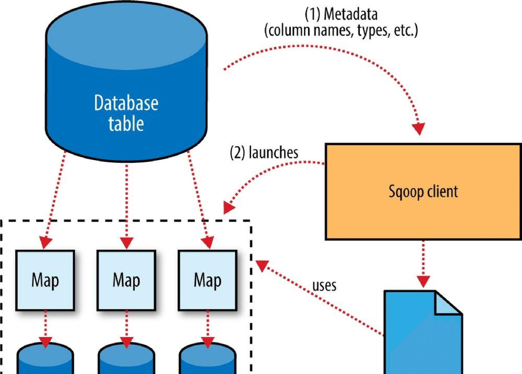

Figure 15-1. Sqoop’s import process
The Widget class from earlier, for example, contains the following methods that retrieve each column from an extracted record:
public Integer getid(); public String get_widget_name(); public java.math.BigDecimal get_price(); public java.sql.Date get_design_date(); public Integer get_version(); public String get_design_comment();
More critical to the import system’s operation, though, are the serialization methods that form the DBWritable interface, which allow the Widget class to interact with JDBC:
public void readFields(ResultSet dbResults) throws SQLException; public void write(PreparedStatement dbStmt) throws SQLException;
JDBC’s ResultSet interface provides a cursor that retrieves records from a query; the readFields() method here will populate the fields of the Widget object with the columns from one row of the ResultSet’s data. The write() method shown here allows Sqoop to insert new Widget rows into a table, a process called _exporting. Exports are discussed in Performing an Export.
The MapReduce job launched by Sqoop uses an InputFormat that can read sections of a table from a database via JDBC. The DataDrivenDBInputFormat provided with Hadoop partitions a query’s results over several map tasks.
Reading a table is typically done with a simple query such as:
SELECT col1,col2,col3,… FROM tableName
But often, better import performance can be gained by dividing this query across multiple nodes. This is done using a splitting column. Using metadata about the table, Sqoop will guess a good column to use for splitting the table (typically the primary key for the table, if one exists). The minimum and maximum values for the primary key column are retrieved, and then these are used in conjunction with a target number of tasks to determine the queries that each map task should issue.
For example, suppose the widgets table had 100,000 entries, with the id column containing values 0 through 99,999. When importing this table, Sqoop would determine that id is the primary key column for the table. When starting the MapReduce job, the DataDrivenDBInputFormat used to perform the import would issue a statement such as SELECT MIN(id), MAX(id) FROM widgets. These values would then be used to interpolate over the entire range of data. Assuming we specified that five map tasks should run in parallel (with -m 5), this would result in each map task executing queries such as
SELECT id, widget_name, … FROM widgets WHERE id >= 0 AND id < 20000,
SELECT id, widget_name, … FROM widgets WHERE id >= 20000 AND id < 40000, and so on.
The choice of splitting column is essential to parallelizing work efficiently. If the id column were not uniformly distributed (perhaps there are no widgets with IDs between 50,000 and 75,000), then some map tasks might have little or no work to perform, whereas others would have a great deal. Users can specify a particular splitting column when running an import job (via the —split-by argument), to tune the job to the data’s actual distribution. If an import job is run as a single (sequential) task with -m 1, this split process is not performed.
After generating the deserialization code and configuring the InputFormat, Sqoop sends the job to the MapReduce cluster. Map tasks execute the queries and deserialize rows from the ResultSet into instances of the generated class, which are either stored directly in SequenceFiles or transformed into delimited text before being written to HDFS.
Controlling the Import
Sqoop does not need to import an entire table at a time. For example, a subset of the table’s columns can be specified for import. Users can also specify a WHERE clause to include in queries via the —where argument, which bounds the rows of the table to import. For example, if widgets 0 through 99,999 were imported last month, but this month our vendor catalog included 1,000 new types of widget, an import could be configured with the clause WHERE id >= 100000; this will start an import job to retrieve all the new rows added to the source database since the previous import run. User-supplied WHERE clauses are applied before task splitting is performed, and are pushed down into the queries executed by each task.
For more control — to perform column transformations, for example — users can specify a —query argument.
Imports and Consistency
When importing data to HDFS, it is important that you ensure access to a consistent snapshot of the source data. (Map tasks reading from a database in parallel are running in separate processes. Thus, they cannot share a single database transaction.) The best way to do this is to ensure that any processes that update existing rows of a table are disabled during the import.
Incremental Imports
It’s common to run imports on a periodic basis so that the data in HDFS is kept synchronized with the data stored in the database. To do this, there needs to be some way of identifying the new data. Sqoop will import rows that have a column value (for the column specified with —check-column) that is greater than some specified value (set via —last-value).
The value specified as —last-value can be a row ID that is strictly increasing, such as an AUTO_INCREMENT primary key in MySQL. This is suitable for the case where new rows are added to the database table, but existing rows are not updated. This mode is called _append _mode, and is activated via —incremental append. Another option is time-based incremental imports (specified by —incremental lastmodified), which is appropriate when existing rows may be updated, and there is a column (the check column) that records the last modified time of the update.
At the end of an incremental import, Sqoop will print out the value to be specified as -last-value on the next import. This is useful when running incremental imports manually, but for running periodic imports it is better to use Sqoop’s saved job facility, which automatically stores the last value and uses it on the next job run. Type sqoop job —help for usage instructions for saved jobs.
Direct-Mode Imports
Sqoop’s architecture allows it to choose from multiple available strategies for performing an import. Most databases will use the DataDrivenDBInputFormat-based approach described earlier. Some databases, however, offer specific tools designed to extract data quickly. For example, MySQL’s mysqldump application can read from a table with greater throughput than a JDBC channel. The use of these external tools is referred to as direct mode in Sqoop’s documentation. Direct mode must be specifically enabled by the user (via the —direct argument), as it is not as general purpose as the JDBC approach. (For example, MySQL’s direct mode cannot handle large objects, such as CLOB or BLOB columns, and that’s why Sqoop needs to use a JDBC-specific API to load these columns into HDFS.)
For databases that provide such tools, Sqoop can use these to great effect. A direct-mode import from MySQL is usually much more efficient (in terms of map tasks and time required) than a comparable JDBC-based import. Sqoop will still launch multiple map tasks in parallel. These tasks will then spawn instances of the mysqldump program and read its output. Sqoop can also perform direct-mode imports from PostgreSQL, Oracle, and Netezza.
Even when direct mode is used to access the contents of a database, the metadata is still queried through JDBC.
Working with Imported Data
Once data has been imported to HDFS, it is ready for processing by custom MapReduce programs. Text-based imports can easily be used in scripts run with Hadoop Streaming or in MapReduce jobs run with the default TextInputFormat.
To use individual fields of an imported record, though, the field delimiters (and any escape/enclosing characters) must be parsed and the field values extracted and converted to the appropriate data types. For example, the ID of the “sprocket” widget is represented as the string “1” in the text file, but should be parsed into an Integer or int variable in Java. The generated table class provided by Sqoop can automate this process, allowing you to focus on the actual MapReduce job to run. Each autogenerated class has several overloaded methods named parse() that operate on the data represented as Text, CharSequence, char[], or other common types.
The MapReduce application called MaxWidgetId (available in the example code) will find the widget with the highest ID. The class can be compiled into a JAR file along with Widget.java using the Maven POM that comes with the example code. The JAR file is called sqoop-examples.jar, and is executed like so:
% HADOOPCLASSPATH=$SQOOP_HOME/sqoop-_version.jar hadoop jar \
> sqoop-examples.jar MaxWidgetId -libjars $SQOOPHOME/sqoop-_version.jar
This command line ensures that Sqoop is on the classpath locally (via
$HADOOPCLASSPATH) when running the MaxWidgetId.run() method, as well as when map tasks are running on the cluster (via the -libjars argument).
When run, the _maxwidget path in HDFS will contain a file named part-r-00000 with the following expected result:
3,gadget,99.99,1983-08-13,13,Our flagship product
It is worth noting that in this example MapReduce program, a Widget object was emitted from the mapper to the reducer; the autogenerated Widget class implements the Writable interface provided by Hadoop, which allows the object to be sent via Hadoop’s serialization mechanism, as well as written to and read from SequenceFiles.
The MaxWidgetId example is built on the new MapReduce API. MapReduce applications that rely on Sqoop-generated code can be built on the new or old APIs, though some advanced features (such as working with large objects) are more convenient to use in the new API.
Avro-based imports can be processed using the APIs described in Avro MapReduce. With the Generic Avro mapping, the MapReduce program does not need to use schema-specific generated code (although this is an option too, by using Avro’s Specific compiler; Sqoop does not do the code generation in this case). The example code includes a program called MaxWidgetIdGenericAvro, which finds the widget with the highest ID and writes out the result in an Avro datafile.
Imported Data and Hive
As we’ll see in Chapter 17, for many types of analysis, using a system such as Hive to handle relational operations can dramatically ease the development of the analytic pipeline. Especially for data originally from a relational data source, using Hive makes a lot of sense. Hive and Sqoop together form a powerful toolchain for performing analysis.
Suppose we had another log of data in our system, coming from a web-based widget purchasing system. This might return logfiles containing a widget ID, a quantity, a shipping address, and an order date.
Here is a snippet from an example log of this type:
1,15,120 Any St.,Los Angeles,CA,90210,2010-08-01
3,4,120 Any St.,Los Angeles,CA,90210,2010-08-01
2,5,400 Some Pl.,Cupertino,CA,95014,2010-07-30
2,7,88 Mile Rd.,Manhattan,NY,10005,2010-07-18
By using Hadoop to analyze this purchase log, we can gain insight into our sales operation. By combining this data with the data extracted from our relational data source (the widgets table), we can do better. In this example session, we will compute which zip code is responsible for the most sales dollars, so we can better focus our sales team’s operations. Doing this requires data from both the sales log and the widgets table.
The table shown in the previous code snippet should be in a local file named sales.log for this to work.
First, let’s load the sales data into Hive:
hive> CREATE TABLE sales(widget_id INT, qty INT, > street STRING, city STRING, state STRING,
> zip INT, sale_date STRING)
> ROW FORMAT DELIMITED FIELDS TERMINATED BY ‘,’;
OK
Time taken: 5.248 seconds
hive> LOAD DATA LOCAL INPATH “ch15-sqoop/sales.log” INTO TABLE sales;
…
Loading data to table default.sales
Table default.sales stats: [numFiles=1, numRows=0, totalSize=189, rawDataSize=0] OK
Time taken: 0.6 seconds
Sqoop can generate a Hive table based on a table from an existing relational data source. We’ve already imported the widgets data to HDFS, so we can generate the Hive table definition and then load in the HDFS-resident data:
% sqoop create-hive-table —connect jdbc:mysql://localhost/hadoopguide \
> —table widgets —fields-terminated-by ‘,’
…
14/10/29 11:54:52 INFO hive.HiveImport: OK
14/10/29 11:54:52 INFO hive.HiveImport: Time taken: 1.098 seconds 14/10/29 11:54:52 INFO hive.HiveImport: Hive import complete.
% hive
hive> LOAD DATA INPATH “widgets” INTO TABLE widgets;
Loading data to table widgets OK
Time taken: 3.265 seconds
When creating a Hive table definition with a specific already imported dataset in mind, we need to specify the delimiters used in that dataset. Otherwise, Sqoop will allow Hive to use its default delimiters (which are different from Sqoop’s default delimiters).
NOTE
Hive’s type system is less rich than that of most SQL systems. Many SQL types do not have direct analogues in Hive. When Sqoop generates a Hive table definition for an import, it uses the best Hive type available to hold a column’s values. This may result in a decrease in precision. When this occurs, Sqoop will provide you with a warning message such as this one:
14/10/29 11:54:43 WARN hive.TableDefWriter: Column design_date had to be cast to a less precise type in Hive
This three-step process of importing data to HDFS, creating the Hive table, and then loading the HDFS-resident data into Hive can be shortened to one step if you know that you want to import straight from a database directly into Hive. During an import, Sqoop can generate the Hive table definition and then load in the data. Had we not already performed the import, we could have executed this command, which creates the widgets table in Hive based on the copy in MySQL:
% sqoop import —connect jdbc:mysql://localhost/hadoopguide \
> —table widgets -m 1 —hive-import
NOTE
Running sqoop import with the —hive-import argument will load the data directly from the source database into Hive; it infers a Hive schema automatically based on the schema for the table in the source database. Using this, you can get started working with your data in Hive with only one command.
Regardless of which data import route we chose, we can now use the widgets dataset and the sales dataset together to calculate the most profitable zip code. Let’s do so, and also save the result of this query in another table for later:
hive> CREATE TABLE zip_profits
> AS
> SELECT SUM(w.price * s.qty) AS sales_vol, s.zip FROM SALES s
> JOIN widgets w ON (s.widget_id = w.id) GROUP BY s.zip;
…
Moving data to: hdfs://localhost/user/hive/warehouse/zip_profits… OK
hive> SELECT * FROM zip_profits ORDER BY sales_vol DESC;
…
OK
403.71 90210
28.0 10005
20.0 95014
Importing Large Objects
Most databases provide the capability to store large amounts of data in a single field.
Depending on whether this data is textual or binary in nature, it is usually represented as a CLOB or BLOB column in the table. These “large objects” are often handled specially by the database itself. In particular, most tables are physically laid out on disk as in Figure 15-2. When scanning through rows to determine which rows match the criteria for a particular query, this typically involves reading all columns of each row from disk. If large objects were stored “inline” in this fashion, they would adversely affect the performance of such scans. Therefore, large objects are often stored externally from their rows, as in Figure 153. Accessing a large object often requires “opening” it through the reference contained in the row.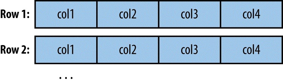
Figure 15-2. Database tables are typically physically represented as an array of rows, with all the columns in a row stored adjacent to one another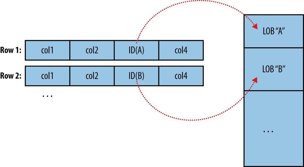
Figure 15-3. Large objects are usually held in a separate area of storage; the main row storage contains indirect references to the large objects
The difficulty of working with large objects in a database suggests that a system such as
Hadoop, which is much better suited to storing and processing large, complex data objects, is an ideal repository for such information. Sqoop can extract large objects from tables and store them in HDFS for further processing.
As in a database, MapReduce typically materializes every record before passing it along to the mapper. If individual records are truly large, this can be very inefficient.
As shown earlier, records imported by Sqoop are laid out on disk in a fashion very similar to a database’s internal structure: an array of records with all fields of a record concatenated together. When running a MapReduce program over imported records, each map task must fully materialize all fields of each record in its input split. If the contents of a large object field are relevant only for a small subset of the total number of records used as input to a MapReduce program, it would be inefficient to fully materialize all these records. Furthermore, depending on the size of the large object, full materialization in memory may be impossible.
To overcome these difficulties, Sqoop will store imported large objects in a separate file called a LobFile, if they are larger than a threshold size of 16 MB (configurable via the sqoop.inline.lob.length.max setting, in bytes). The LobFile format can store individual records of very large size (a 64-bit address space is used). Each record in a LobFile holds a single large object. The LobFile format allows clients to hold a reference to a record without accessing the record contents. When records are accessed, this is done through a java.io.InputStream (for binary objects) or java.io.Reader (for characterbased objects).
When a record is imported, the “normal” fields will be materialized together in a text file, along with a reference to the LobFile where a CLOB or BLOB column is stored. For example, suppose our widgets table contained a BLOB field named schematic holding the actual schematic diagram for each widget.
An imported record might then look like:
2,gizmo,4.00,2009-11-30,4,null,externalLob(lf,lobfile0,100,5011714)
The externalLob(…) text is a reference to an externally stored large object, stored in LobFile format (lf) in a file named lobfile0, with the specified byte offset and length inside that file.
When working with this record, the Widget.get_schematic() method would return an object of type BlobRef referencing the schematic column, but not actually containing its contents. The BlobRef.getDataStream() method actually opens the LobFile and returns an InputStream, allowing you to access the schematic field’s contents.
When running a MapReduce job processing many Widget records, you might need to access the schematic fields of only a handful of records. This system allows you to incur the I/O costs of accessing only the required large object entries — a big savings, as individual schematics may be several megabytes or more of data.
The BlobRef and ClobRef classes cache references to underlying LobFiles within a map task. If you do access the schematic fields of several sequentially ordered records, they will take advantage of the existing file pointer’s alignment on the next record body.
Performing an Export
In Sqoop, an import refers to the movement of data from a database system into HDFS. By contrast, an export uses HDFS as the source of data and a remote database as the destination. In the previous sections, we imported some data and then performed some analysis using Hive. We can export the results of this analysis to a database for consumption by other tools.
Before exporting a table from HDFS to a database, we must prepare the database to receive the data by creating the target table. Although Sqoop can infer which Java types are appropriate to hold SQL data types, this translation does not work in both directions (for example, there are several possible SQL column definitions that can hold data in a
Java String; this could be CHAR(64), VARCHAR(200), or something else entirely). Consequently, you must determine which types are most appropriate.
We are going to export the zipprofits table from Hive. We need to create a table in MySQL that has target columns in the same order, with the appropriate SQL types:
% mysql hadoopguide
mysql> CREATE TABLE sales_by_zip (volume DECIMAL(8,2), zip INTEGER); Query OK, 0 rows affected (0.01 sec) Then we run the export command:
% sqoop export —connect jdbc:mysql://localhost/hadoopguide -m 1 \ > —table sales_by_zip —export-dir /user/hive/warehouse/zip_profits \
> —input-fields-terminated-by ‘\0001’
…
14/10/29 12:05:08 INFO mapreduce.ExportJobBase: Transferred 176 bytes in 13.5373 seconds (13.0011 bytes/sec)
14/10/29 12:05:08 INFO mapreduce.ExportJobBase: Exported 3 records.
Finally, we can verify that the export worked by checking MySQL:
% mysql hadoopguide -e ‘SELECT * FROM sales_by_zip’
+————+———-+
| volume | zip |
+————+———-+
| 28.00 | 10005 |
| 403.71 | 90210 |
| 20.00 | 95014 | +————+———-+
When we created the zip_profits table in Hive, we did not specify any delimiters. So Hive used its default delimiters: a Ctrl-A character (Unicode 0x0001) between fields and a newline at the end of each record. When we used Hive to access the contents of this table (in a SELECT statement), Hive converted this to a tab-delimited representation for display on the console. But when reading the tables directly from files, we need to tell Sqoop which delimiters to use. Sqoop assumes records are newline-delimited by default, but needs to be told about the Ctrl-A field delimiters. The —input-fields-terminated-by argument to sqoop export specified this information. Sqoop supports several escape sequences, which start with a backslash () character, when specifying delimiters.
In the example syntax, the escape sequence is enclosed in single quotes to ensure that the shell processes it literally. Without the quotes, the leading backslash itself may need to be escaped (e.g., —input-fields-terminated-by \0001). The escape sequences supported by Sqoop are listed in Table 15-1.
_Table 15-1. Escape sequences that can be used to specify nonprintable characters as field and record delimiters in Sqoop
Escape Description
| \b | Backspaces. |
|---|---|
| \n | Newline. |
| \r | Carriage return. |
| \t | Tab. |
| \‘ | Single quote. |
| \“ | Double quote. |
| \\ | Backslash. |
| \0 | NUL. This will insert NUL characters between fields or lines, or will disable enclosing/escaping if used for one of the —enclosed-by, —optionally-enclosed-by, or —escaped-by arguments. |
| \0ooo | The octal representation of a Unicode character’s code point. The actual character is specified by the octal value ooo. |
| \0xhhh | The hexadecimal representation of a Unicode character’s code point. This should be of the form \0x_, where _hhh is the hex value. For example, —fields-terminated-by ‘\0x10’ specifies the carriage return character. |
Exports: A Deeper Look
The Sqoop performs exports is very similar in nature to how Sqoop performs imports (see Figure 15-4). Before performing the export, Sqoop picks a strategy based on the database connect string. For most systems, Sqoop uses JDBC. Sqoop then generates a Java class based on the target table definition. This generated class has the ability to parse records from text files and insert values of the appropriate types into a table (in addition to the ability to read the columns from a ResultSet). A MapReduce job is then launched that reads the source datafiles from HDFS, parses the records using the generated class, and executes the chosen export strategy.
The JDBC-based export strategy builds up batch INSERT statements that will each add multiple records to the target table. Inserting many records per statement performs much better than executing many single-row INSERT statements on most database systems. Separate threads are used to read from HDFS and communicate with the database, to ensure that I/O operations involving different systems are overlapped as much as possible.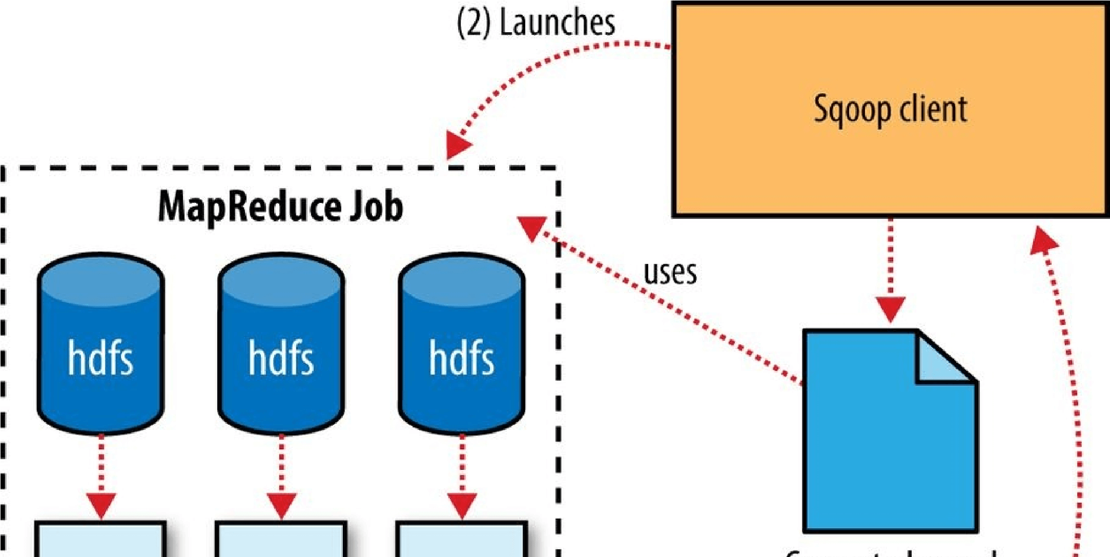
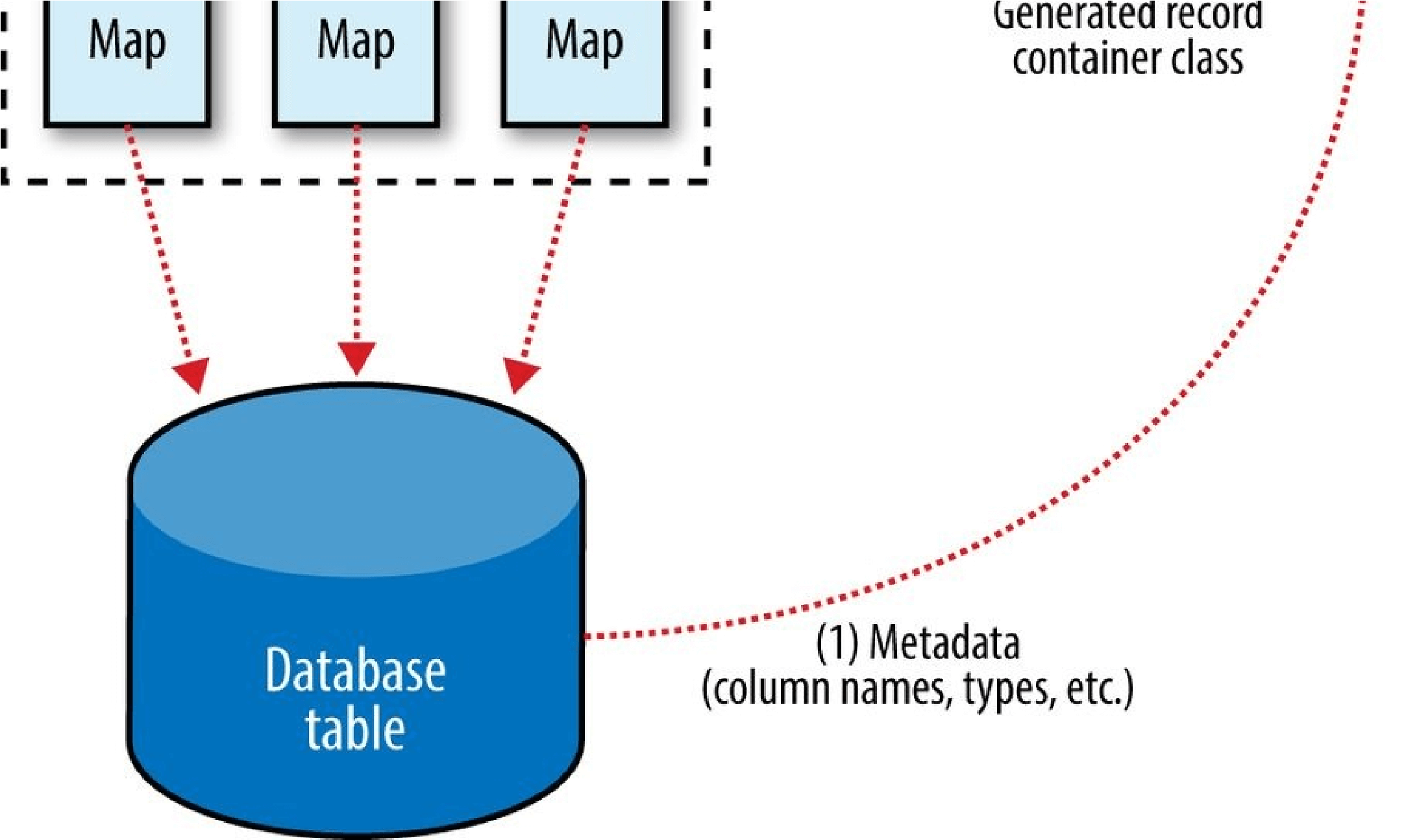
Figure 15-4. Exports are performed in parallel using MapReduce
For MySQL, Sqoop can employ a direct-mode strategy using mysqlimport. Each map task spawns a mysqlimport process that it communicates with via a named FIFO file on the local filesystem. Data is then streamed into mysqlimport via the FIFO channel, and from there into the database.
Whereas most MapReduce jobs reading from HDFS pick the degree of parallelism (number of map tasks) based on the number and size of the files to process, Sqoop’s export system allows users explicit control over the number of tasks. The performance of the export can be affected by the number of parallel writers to the database, so Sqoop uses the CombineFileInputFormat class to group the input files into a smaller number of map tasks.
Exports and Transactionality
Due to the parallel nature of the process, often an export is not an atomic operation. Sqoop will spawn multiple tasks to export slices of the data in parallel. These tasks can complete at different times, meaning that even though transactions are used inside tasks, results from one task may be visible before the results of another task. Moreover, databases often use fixed-size buffers to store transactions. As a result, one transaction cannot necessarily contain the entire set of operations performed by a task. Sqoop commits results every few thousand rows, to ensure that it does not run out of memory. These intermediate results are visible while the export continues. Applications that will use the results of an export should not be started until the export process is complete, or they may see partial results.
To solve this problem, Sqoop can export to a temporary staging table and then, at the end of the job — if the export has succeeded — move the staged data into the destination table in a single transaction. You can specify a staging table with the —staging-table option. The staging table must already exist and have the same schema as the destination. It must also be empty, unless the —clear-staging-table option is also supplied.
NOTE
Using a staging table is slower, since the data must be written twice: first to the staging table, then to the destination table. The export process also uses more space while it is running, since there are two copies of the data while the staged data is being copied to the destination.
Exports and SequenceFiles
The example export reads source data from a Hive table, which is stored in HDFS as a delimited text file. Sqoop can also export delimited text files that were not Hive tables. For example, it can export text files that are the output of a MapReduce job.
Sqoop can export records stored in SequenceFiles to an output table too, although some restrictions apply. A SequenceFile cannot contain arbitrary record types. Sqoop’s export tool will read objects from SequenceFiles and send them directly to the
OutputCollector, which passes the objects to the database export OutputFormat. To work with Sqoop, the record must be stored in the “value” portion of the SequenceFile’s keyvalue pair format and must subclass the org.apache.sqoop.lib.SqoopRecord abstract class (as is done by all classes generated by Sqoop).
If you use the codegen tool (sqoop-codegen) to generate a SqoopRecord implementation for a record based on your export target table, you can write a MapReduce program that populates instances of this class and writes them to SequenceFiles. sqoop-export can then export these SequenceFiles to the table. Another means by which data may be in SqoopRecord instances in SequenceFiles is if data is imported from a database table to HDFS and modified in some fashion, and then the results are stored in SequenceFiles holding records of the same data type.
In this case, Sqoop should reuse the existing class definition to read data from
SequenceFiles, rather than generating a new (temporary) record container class to perform the export, as is done when converting text-based records to database rows. You can suppress code generation and instead use an existing record class and JAR by providing the —class-name and —jar-file arguments to Sqoop. Sqoop will use the specified class, loaded from the specified JAR, when exporting records.
In the following example, we reimport the widgets table as SequenceFiles, and then export it back to the database in a different table:
% sqoop import —connect jdbc:mysql://localhost/hadoopguide \
> —table widgets -m 1 —class-name WidgetHolder —as-sequencefile \
> —target-dir widget_sequence_files —bindir .
…
14/10/29 12:25:03 INFO mapreduce.ImportJobBase: Retrieved 3 records.
% mysql hadoopguide
mysql> CREATE TABLE widgets2(id INT, widget_name VARCHAR(100),
-> price DOUBLE, designed DATE, version INT, notes VARCHAR(200)); Query OK, 0 rows affected (0.03 sec) mysql> exit;
% sqoop export —connect jdbc:mysql://localhost/hadoopguide \
> —table widgets2 -m 1 —class-name WidgetHolder \
> —jar-file WidgetHolder.jar —export-dir widget_sequence_files
…
14/10/29 12:28:17 INFO mapreduce.ExportJobBase: Exported 3 records.
During the import, we specified the SequenceFile format and indicated that we wanted the JAR file to be placed in the current directory (with —bindir) so we can reuse it. Otherwise, it would be placed in a temporary directory. We then created a destination table for the export, which had a slightly different schema (albeit one that is compatible with the original data). Finally, we ran an export that used the existing generated code to read the records from the SequenceFile and write them to the database.
Further Reading
For more information on using Sqoop, consult the Apache Sqoop Cookbook by Kathleen Ting and Jarek Jarcec Cecho (O’Reilly, 2013).
[94] Of course, in a production deployment we’d need to be much more careful about access control, but this serves for demonstration purposes. The grant privilege shown in the example also assumes you’re running a pseudodistributed Hadoop instance. If you’re working with a distributed Hadoop cluster, you’d need to enable remote access by at least one user, whose account would be used to perform imports and exports via Sqoop.
[95] Available from the Apache Software Foundation website.

若有收获,就点个赞吧
0 人点赞
