学习起始时间：20220414。将点云技术应用与CAE模型设计优化，应该是一个不错的方向。

点云学习资料

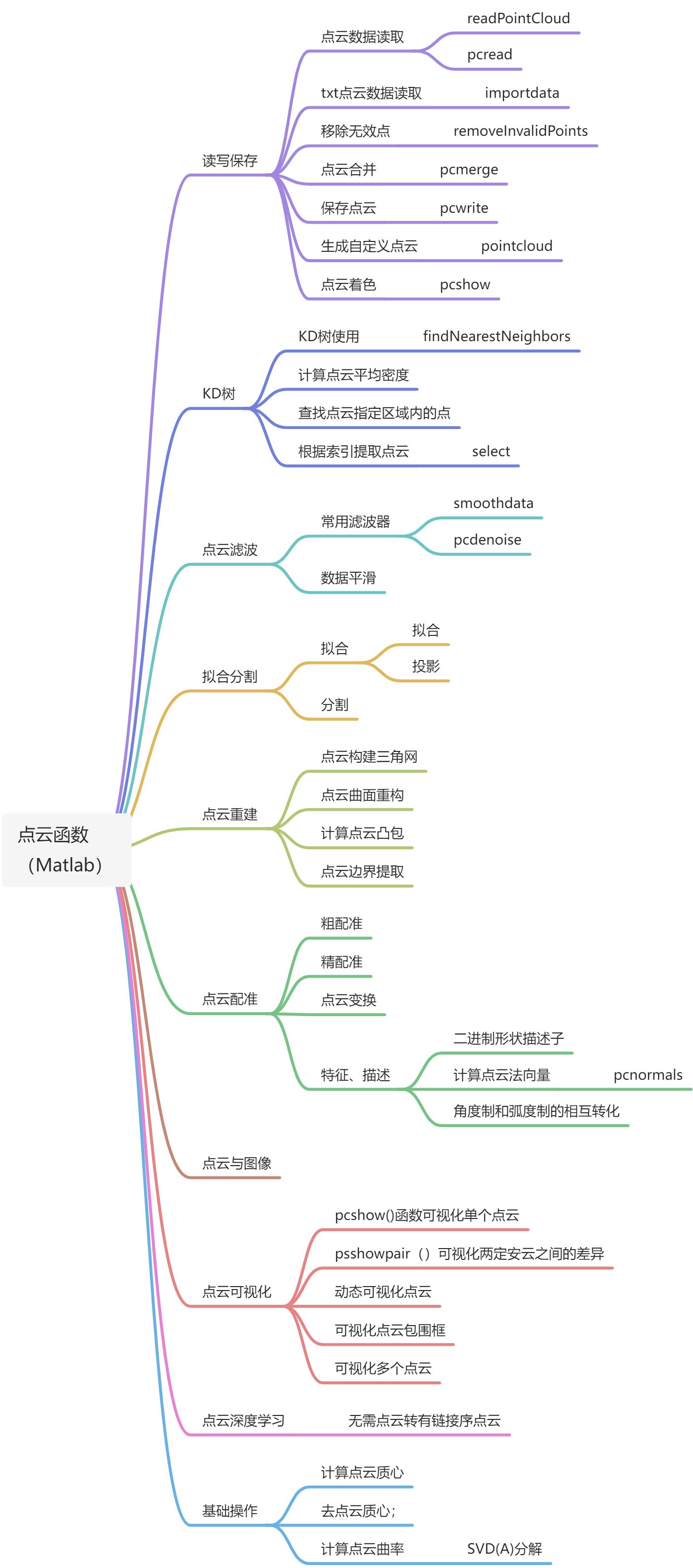
点云处理常用函数（Matlab）

网络素材

总概

点云读取与保存

txt格式转化为pcd格式，是点云数据处理的第一步；

点云特征识别

点云滤波

参考书籍

点云库PCL学习教程.pdf

参考文献

点云数据处理与特征识别关键技术研究_李自胜.pdf
基于邻域表面形变信息加权的点云配准_李新春; 闫振宇; 林森.pdf
基于特征提取的点云自动配准优化研究_杨高朝.pdf
散乱数据点的k近邻搜索算法_刘晓东; 刘国荣; 王颖; 席延军.pdf
适用于激光点云配准的重叠区域提取方法_王帅; 孙华燕; 郭惠超.pdf
一种基于高斯映射的三维点云特征线提取方法_徐卫青; 陈西江; 章光; 袁俏俏.pdf
一种基于特征提取的点云自动配准算法_黄源; 达飞鹏; 陶海跻.pdf

研究策划

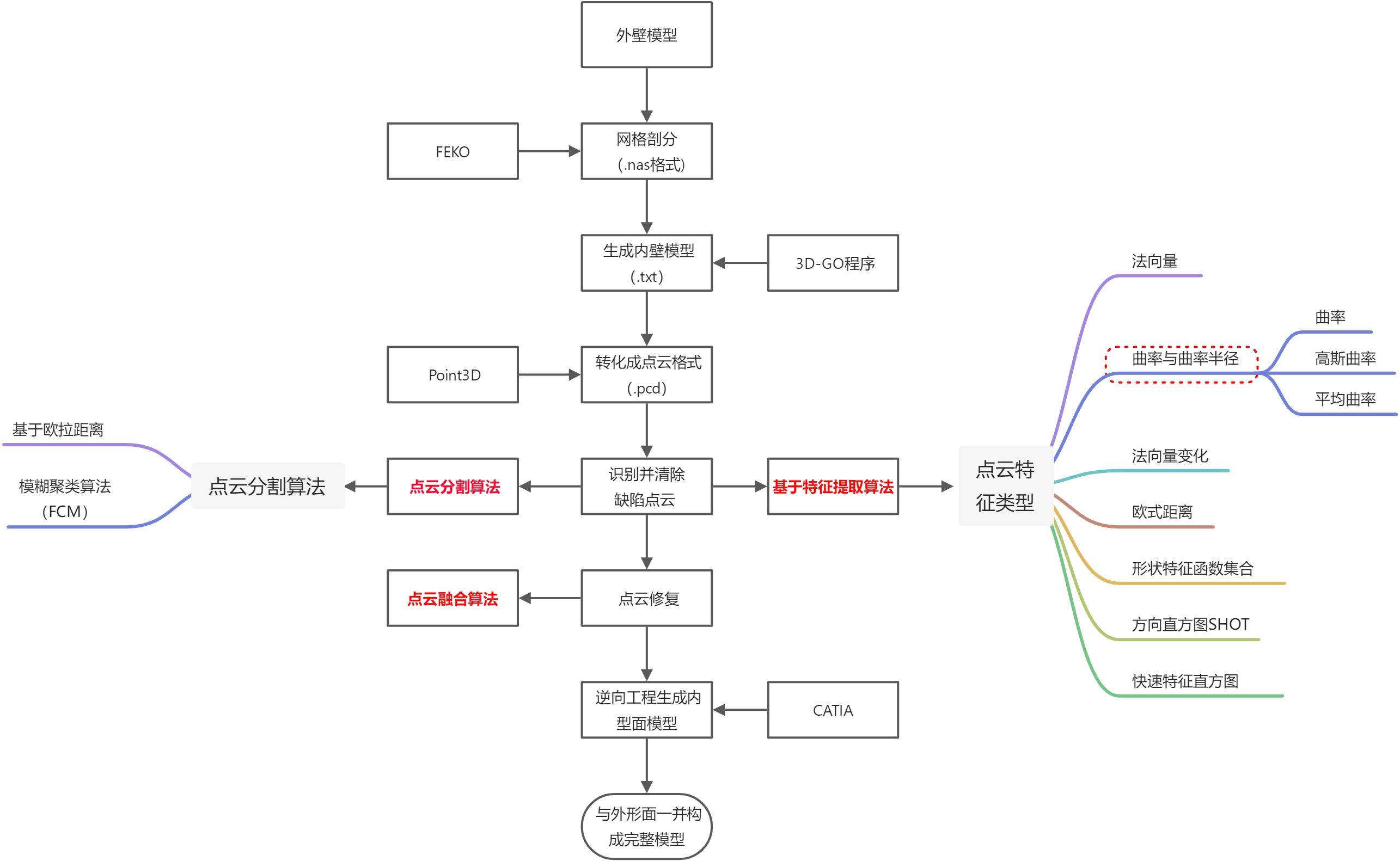
研究方案（技术路线）

关键技术梳理

目前要解决的技术问题的主要技术难点：

1. 依据外壁模型结合几何光学生成内壁初步点云；
2. 缺陷点云的识别、分割与清理；
3. 依据模型要求进行自适应融合。

   关键技术攻关参考

   点云特征识别

   其中缺陷点云的修复就涉及到点云的特征识别和提取的问题：

   点云分割

   大规模点云模型几何造型技术研究_邹万红.pdf
   点云模型分割与融合关键技术研究_孙金虎.pdf
   基于边特征的点云数据区域分割_柯映林; 单东日.pdf

   点云融合

深度学习方法

deep learning on point sets for 3D classification and segmentation.pdf
基于深度学习的点云分割方法综述.pdf
基于深度学习的点云分割算法的研究_魏梦如.pdf

关键技术攻关

step1:基于3D-GO的内型面生成

该模块分为两个部分：1）主程序为3D-GO，依据外壁模型，基于平均入射角和壁厚计算公式，生成内壁点云模型；2）read_meshfile，网格读取函数，读取.nas网格，并返回主程序所需网格信息。

%*********************************软件需求********************************
%3）网格读取函数需要设置变量，可读取任意网格数据;
%4）具备可视化的功能，将管束照射到的面元可视化，2种图：1）颜色与照射密度有关；2）颜色与入射角有关;
%5）能够依据设置，自动建立头部内倒角；
%6）具备异形夹层结构天线罩的快速建模；
%***********************************存在问题******************************
%2）架构还很混乱，循环太多，速度太慢，需要进行去耦和模块化;
%*************************************************************************
clear;clc;close all;
%%
%*************求解设置**************
freq=17;%频率（GHz）
lambda=300/freq;%波长（mm）
Er=3.1;%介质介电常数
R=150;%天线口径
a=0.1;%天线孔径面边缘照射系数
%%
%读取网格
[geomesh]=read_meshfile_nas(); %读取网格信息（triangle：每个三角面元的节点编号；...
                               ...nodes:每个节点的坐标；tri_area:三角面元的面积；
                               ...inc_pos：三角面元的中心点坐标；normal_outter:
                               ...三角面元法向量坐标）
geomesh.inc_pos=1000*geomesh.inc_pos;     %三角面元中心点坐标等比例放大
geomesh.Nodes=1000.*geomesh.Nodes;        %三角面元节点尺寸等比列放大
Reverse=[1;1;1]*geomesh.norm_outter(3,:)./abs(geomesh.norm_outter(3,:));%定义网格法向变换矩阵
geomesh.norm_outter=geomesh.norm_outter.*Reverse; %将三角面元法向量统一为外法向量
% figure(3);%外型面绘图
% scatter3(geomesh.inc_pos(1,:),geomesh.inc_pos(2,:),geomesh.inc_pos(3,:),'+');
%%
%*************天线口面发出的管束对罩体三角元进行遍历*******************
theta1=zeros(1,length(geomesh.Triangles));%划分空间，存储不同面元处的平均入射角
thick=zeros(1,length(geomesh.Triangles)); %划分空间，存储不同面元处的壁厚
th_sum=zeros(1,length(geomesh.Triangles));%划分空间，记录每个三角面元的总入射角(按功率加权)
p_sum=zeros(1,length(geomesh.Triangles)); %划分空间，记录每个三角面元的总入射功率
%外循环为天线波束指向的扫描
th_max=zeros(1,533);%检查管线与面元法向量夹角是否满足要求
t=0;
for theta=0:1:40
    for phi=0:30:360
        Rot_y=[cos(theta*pi/180) 0 sin(theta*pi/180);0 1 0;sin(theta*pi/180) 0 cos(theta*pi/180)];%绕y轴旋转theta的旋转矩阵
        Rot_z=[cos(phi*pi/180) -sin(phi*pi/180) 0;sin(phi*pi/180) cos(phi*pi/180) 0; 0 0 1];%绕z轴旋转phi的旋转矩阵
        P=zeros(1,length(geomesh.Triangles));%划分空间，临时存放每个三角面元的在不同扫描角下的功率
        inc_theta=zeros(1,length(geomesh.Triangles));%划分空间，临时存放每个三角面元不同扫描角下的入射角下(按功率加权)
        k_source=[0,0,1]*Rot_y*Rot_z;%天线源发出的管线转动
        %内循环为三角面元的遍历
        x1=[0 0 0];       %取管束中线上的两个点x1,x2
        x2=k_source;
        for m=1:1:length(geomesh.Triangles)
            x0=[geomesh.inc_pos(1,m) geomesh.inc_pos(2,m) geomesh.inc_pos(3,m)];%取三角面元上中点为线外点
            d=norm(cross((x0-x1),(x0-x2)))/norm(x2-x1);
            if d<=R&&dot((x0-x1),(x2-x1))>0
              P(m)=(a+(1-a)*(sin(pi/2*(1-d/R)))^2)^2;
              inc_theta(m) = acosd(dot(k_source,geomesh.norm_outter(:,m)));
            end
        end
%         if max(inc_theta)>=90
%             [ii,jj]=[theta,phi];
%         end
        p_sum=p_sum+P;%不同扫描角下的三角面元照射功率累加
        th_sum=th_sum+ P.*inc_theta;%不同扫描角下的三角面元入射角累加（加权）
    end
end
[thh_max,p]=max(th_max);
%%
%计算平均入射角并生成内型面散点geomesh
inner_pos=zeros(3,m);%划分空间，存放内型面数据
for m=1:length(geomesh.Triangles)
    if p_sum(m)~=0      %入射功率非零，利用公式计算壁厚
        theta1(m)=th_sum(m)/p_sum(m);    %计算入射角的加权平均
    end
    thick(m)=1*lambda/(2*sqrt(Er-(sin(theta1(m)*pi/180))^2));  %依据平均入射角，按照公式计算最优壁厚
    inner_pos(:,m)=geomesh.inc_pos(:,m)-thick(m).*geomesh.norm_outter(:,m);%平移生成内型面散点
end
meshplot(geomesh.Triangles,geomesh.Nodes,theta1);
meshplot(geomesh.Triangles,geomesh.Nodes,p_sum);
meshplot(geomesh.Triangles,geomesh.Nodes,thick);
xlabel('x');
ylabel('y');
zlabel('z');
figure(4);%内型面绘图
scatter3(inner_pos(1,:),inner_pos(2,:),inner_pos(3,:),'o');
inner_pos=inner_pos';
save C:\Users\em.liu\Desktop\GO_3D\SR_58_1_inner_pos.txt -ascii inner_pos;%数据保存为txt格式

%%read_meshfile，读取.nas网格，并生成相关参数
function [geomesh]=read_meshfile_nas()
%READ_MESHFILE_NAS 此处显示有关此函数的摘要
%函数输出一个结构体geomesh
%geomesh.Triangles:
%geomesh.Nodes:
%geomesh.tri_area:网格面积
%geomesh.inc_pos:网格中心坐标
% geomesh.norm_outter:网格外法向
% geomesh.ntri:网格数目
%   此处显示详细说明
% outputArg1 = inputArg1;
% outputArg2 = inputArg2;
global nNode
filepath='C:\Users\em.liu\Desktop\GO_3D\';
filename='SR_58_1.nas';
unit_Length=1e-3;
fid=fopen([filepath,filename]);
% linetmp=1;
nNode=0;
while ~feof(fid)
    txtline=fgetl(fid);
    if contains(txtline,'GRID*')
        nNode=nNode+1;    
    end
end
fclose(fid);
fid=fopen([filepath,filename]);
vision= fgetl(fid); % 版本消息
null  = fgetl(fid);   % 
null  = fgetl(fid);   % 文件名
null  = fgetl(fid);   % 日期
null  = fgetl(fid);   % 
null  = fgetl(fid);   % 线段个数
ntri  = fgetl(fid);   % 三角形个数
ntri  = str2double(ntri(isstrprop(ntri,'digit')));
ncube = fgetl(fid);
ntetr = fgetl(fid);
Nodes = zeros(nNode,3);
Triangles = zeros(ntri,3);
for ii=1:nNode
    s1=fgetl(fid);
%     s1tmp=textscan(s1,'%f','delimiter',' ');
    Nodes(str2double(s1(20:24)),1:2)=[str2double(s1(40:56)),str2double(s1(57:72))];
    s2=fgetl(fid);
    Nodes(str2double(s1(20:24)),3)=str2double(s2(9:end));
end
for ii=1:ntri
    s3=fgetl(fid);
    s3tmp=regexp(s3,'\d*','match');
    Triangles(str2double(s3tmp(2)),:)=str2double([s3tmp(4:6)]);
end
clear s1 s2 s3 s3tmp null;
Triangles=Triangles.';
Nodes=Nodes.'*unit_Length;
fclose(fid);
%% 求三角形面元的法向量
s_norm=zeros(3,ntri);
tri_area=zeros(1,ntri);
inc_pos=zeros(3,ntri);
for ii=1:ntri
    s_norm(:,ii)=cross((Nodes(:,Triangles(2,ii))-Nodes(:,Triangles(1,ii))),(Nodes(:,Triangles(1,ii))-Nodes(:,Triangles(3,ii))));
end
norm_outter=s_norm./repmat(sqrt(sum(s_norm.^2)),3,1);
for ii=1:ntri
    v1=(Nodes(:,Triangles(2,ii))-Nodes(:,Triangles(1,ii))).';
    v2=(Nodes(:,Triangles(3,ii))-Nodes(:,Triangles(1,ii))).';
    v3=cross(v1,v2)/norm(cross(v1,v2));
    tri_area(ii)=0.5*det([v1;v2;v3]);  % 三角形面积
    inc_pos(:,ii)=1/3*(Nodes(:,Triangles(1,ii))+Nodes(:,Triangles(2,ii))+Nodes(:,Triangles(3,ii)));
end
geomesh.Triangles=Triangles;
geomesh.Nodes=Nodes;
geomesh.tri_area=tri_area;
geomesh.inc_pos=inc_pos;
geomesh.norm_outter=norm_outter;
geomesh.ntri=ntri;
%end

step2:点云生成

将.txt的点云文件转化成通用点云格式.pcd。

%%将txt格式的数据转化为pcd格式的数据
pcData=load("SR_58_1_inner_pos.txt");
ptCloud = pointCloud(pcData(:,1:3));
pcwrite(ptCloud, 'SR_58_1.pcd', 'Encoding', 'ascii'); %将程序中的xyz数据写入pcd文件中
pc = pcread('SR_58_1.pcd');
pcshow(pc); %显示点云

step3:点云特征识别

点云的特征主要分为一下几种：1）法向量以及法向量的变化；2）曲率以及曲率半径，其中曲率主要又分为三种形式：基于KNN计算的曲率，以及高斯曲率和平均曲率；3）欧式距离；4）形状特征函数集合ESF；4）方向直方图SHOT；5）快速特征直方图FPFH。不同类型的点云的使用场合也有所区别。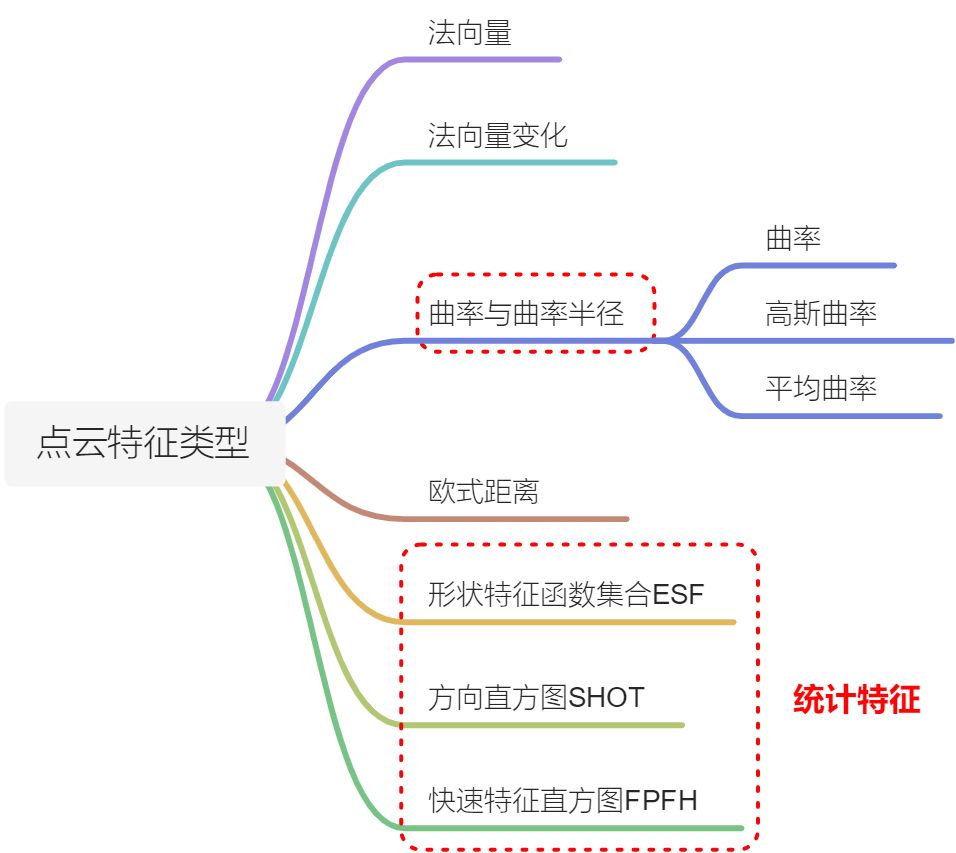

法向量

参考资料：
程序包含两部分：1）主程序为EV_demo；2）EV函数，计算法向量的函数。

A = load('inner_pos.txt');
[M,~] = size(A);
data = A; 
normal = zeros(M,3);
EVs = zeros(M,3);
k = 15;
idx = knnsearch(data,data,'Distance','euclidean','NSMethod','kdtree','K',k); 
for i = 1:M
    %%% 当前点邻域点集索引
    idx_cur = idx(i,2:end);  
    %%% 当前点邻域点集
    knb_pts = data(idx_cur,1:3);
    [normal(i,:),EVs(i,:)] = EV(knb_pts);
end
normal(find(normal(:,3)<0),:) = -normal(find(normal(:,3)<0),:);
figure;
scatter3(data(:,1),data(:,2),data(:,3),20,'k','filled')
hold on
quiver3(data(:,1),data(:,2),data(:,3),normal(:,1),normal(:,2),normal(:,3),'r')
axis equal vis3d

function [normal_vector,EVs] = EV(knbpts)
% knbpts：邻近点
% normal_vector:单位法向量
% EVs ：单位特征值
P = knbpts(:,1:3);
[m,~] = size(P);
% 计算协方差矩阵
P = P-ones(m,1)*(sum(P,1)/m);
C = P.'*P./(m-1);  
% 计算特征值与特征向量
[V, D] = eig(C);
% 最小特征值对应的特征向量为法向量
s1 = D(1,1);
s2 = D(2,2);
s3 = D(3,3);
if (s1 <= s2 && s1 <= s3)
    normal_vector(1,:) = V(:,1)/norm(V(:,1));
elseif (s2 <= s1 && s2 <= s3)
    normal_vector(1,:) = V(:,2)/norm(V(:,2));
elseif (s3 <= s1 && s3 <= s2)
    normal_vector(1,:) = V(:,3)/norm(V(:,3));
end 
% 单位特征值
epsilon_to_add = 1e-8;
% EVs(1) > EVs(2) > EVs(3)
EVs(1,:) = [D(3,3) D(2,2) D(1,1)];
if EVs(1,3) <= 0
    EVs(1,3) = epsilon_to_add;
    if EVs(1,2) <= 0
        EVs(1,2) = epsilon_to_add;
        if EVs(1,1) <= 0
            EVs(1,1) = epsilon_to_add;
        end
    end
end
sum_EVs = EVs(1) + EVs(2) + EVs(3);    
EVs = EVs/sum_EVs;
end

暂时未想到直接使用法向量进行点云特征识别的技术方案。

法向量变化

法向量无法直接作为特征对点云的棱边和驻点进行识别，但是法向量的变化却可以作为的特征进行识别。在棱边和驻点区域，点云曲率大，相应的法向量的变化也会更加剧烈，这种特征识别方法预计会与基于曲率的特征识别具有相同的效果和缺陷。

曲率

基于如下参考内容的代码实现：
在源代码的基础上，调整了点云显示的colorbar（defaut->hot），点云特征显示的更加明显。

clc;
clear;
%% -------------------------加载点云数据---------------------------------
ptCloud = pcread('SR_58_1.pcd');
%% -------------------------获取点的坐标---------------------------------
x=ptCloud.Location(:,1);
y=ptCloud.Location(:,2);
z=ptCloud.Location(:,3);
P=[x,y,z];
%% -----------------------计算每个点的曲率-------------------------------
K=20;                           % k邻域点的个数
curvature = zeros(length(x),1); % 保存曲率结果的数组
Radi=NaN(length(x),1);
for i = 1:length(x)             % 遍历计算每一个点  
    point=P(i,:);
%   [indices,dists] = findNearestNeighbors(ptCloud,point,K,'sort',true);%k近邻搜索
    [indices,dists] = findNearestNeighbors(ptCloud,point,K);%k近邻搜索
    % 1、获取近邻点坐标
    nnpoint=P(indices,:);
    % 2、计算邻域点的质心
    centroid = mean(nnpoint,1);
    % 3、去质心化
    deMean = bsxfun(@minus,nnpoint,centroid);
    % 4、构建协方差矩阵
    H = 1/length(indices)*(deMean'*deMean);
    % 5、奇异值分解计算特征值
    s = svd(H);
    % 6、计算表面曲率
    curvature(i) = s(3)/sum(s);
%% --------通过对曲率设置阈值，清除缺陷点云----------
    if curvature(i)>=0.1
        x(i)=NaN;
        y(i)=NaN;
        z(i)=NaN;
        curvature(i)=NaN;
    end
end
%% -------------------按曲率大小进行颜色渲染-----------------------------
scatter3(x,y,z,3,curvature,'filled');
colorbar;
colormap hot;
title("按曲率大小进行颜色渲染");
% hoid on;
% scatter3(x,y,z,3,Radi,'filled');
% colorbar;
% title("按曲率半径大小进行颜色渲染");

目前基于曲率作为点云特征对内型面点云进行识别，通过调节点云密度（网格密度）和K领域点数目以及曲率阈值，基本能实现对棱边和驻点区域的识别。

存在的问题：1）棱边交叠的冗余部分不能完全识别到，为后续点云清理带来麻烦；2）采用曲率特征，棱边和驻点的外形特征无法做到有效区分。

K-H（基于MLS算法）

基于KNN的曲率计算方法，可以对棱边和驻点一并识别出来，但是却无法对棱边和驻点的形状特征进行区分，而K-H分类方法可以对棱边的“脊特征”和驻点的“峰特征”进行区分，叠加上文的曲率特征识别方法，是否可以对驻点和棱边进行二次区分。
实现代码
输出结果为高斯曲率和主曲率，代码包括主程序MLS_demo和调用函数（nearestneighbour、MLS_projection、MLS_curvature_computing、MLS_energy）。目前最大的问题是尚未明确任意散乱点云如何嵌入该代码中，无法直接将该代码应用起来。

% function MLS_demo(MLS:moving least squares,移动最小二乘法)
% Demo for direct computing of point-set surface curvatures
% Created : Sep. 29, 2007
% Version : 1.0
% Matlab Version : 7.0 ( Windows )
% %%%%%%%%%%%%%%%%%%%%%%%%%%%%%%%%%%%%%%%%%%%%%%%%%%%%%%%%%%%%%%%%
number_of_neighbor = 90;
gaussian_param = 0.06;
% read the input synthetic/real point data and normals
file_name_for_input = 'demo_input_data.txt';
fp = fopen(file_name_for_input, 'r');
points = fscanf(fp,'%f');
bluff_data = (reshape(points,6,size(points,1)/6))';
fclose(fp);
x = bluff_data(:,1);     %前三个为点云坐标
y = bluff_data(:,2);
z = bluff_data(:,3);
normal_x = bluff_data(:,4);  %后三个为点云法向量
normal_y = bluff_data(:,5);
normal_z = bluff_data(:,6);
input_pnts = [x';y';z'];
input_normals = [normal_x';normal_y';normal_z'];
% read the evaluation point data
file_name_for_evaluation = 'SR_58_1_inner_pos.txt';
fp = fopen(file_name_for_evaluation, 'r');
points = fscanf(fp,'%f');
bluff_data = (reshape(points,3,size(points,1)/3))';
fclose(fp);
x = bluff_data(:,1);
y = bluff_data(:,2);
z = bluff_data(:,3);
eval_pnts = [x';y';z'];
% Project a point onto the MLS surface defined by input points  
for i = size(eval_pnts,2)
    eval_pnts(:,i) = MLS_projection(input_pnts, input_normals, eval_pnts(:,i), number_of_neighbor, gaussian_param);
end
% Direct computing of point-set surface curvatures  
[gaussian, mean, k1, k2] = MLS_curvature_computing(input_pnts, input_normals, eval_pnts, number_of_neighbor, gaussian_param);
% save the resulting curvatures
file_name_for_evaluation = 'demo_resulting_curvatures.txt';
fp = fopen('demo_resulting_curvatures.txt', 'w+');
for i = 1:size(eval_pnts,2)
    fprintf(fp,'%f %f %f %f\n', gaussian(i), mean(i), k1(i), k2(i));
end
fclose(fp);
figure(1);
scatter3(x,y,z,3,gaussian,'filled');
colorbar;
colormap hot;
title("高斯曲率");
figure(2);
scatter3(x,y,z,3,mean,'filled');
colorbar;
colormap hot;
title("主曲率");

function [idx, tri] = nearestneighbour(varargin)
%NEARESTNEIGHBOUR    find nearest neighbours
%   IDX = NEARESTNEIGHBOUR(P, X) finds the nearest neighbour by Euclidean
%   distance to each point in P from X. P and X are both matrices with the
%   same number of rows, and points are the columns of the matrices. Output
%   is a vector of indices into X such that X(:, IDX) are the nearest
%   neighbours to P
%
%   IDX = NEARESTNEIGHBOUR(I, X) where I is a logical vector or vector of
%   indices, and X has at least two rows, finds the nearest neighbour in X
%   to each of the points X(:, I).
%   I must be a row vector to distinguish it from a single point.
%   If X has only one row, the first input is treated as a set of 1D points
%   rather than a vector of indices
%
%   IDX = NEARESTNEIGHBOUR(..., Property, Value)
%   Calls NEARESTNEIGHBOUR with the indicated parameters set.
%      Property:                         Value:
%      ---------                         ------  
%         NumberOfNeighbours             natural number, default 1
%            NEARESTNEIGHBOUR(..., 'NumberOfNeighbours', K) finds the closest
%            K points in ascending order to each point, rather than the
%            closest point
%
%         DelaunayMode                   {'on', 'off', |'auto'|}
%            DelaunayMode being set to 'on' means NEARESTNEIGHBOUR uses the
%            a Delaunay triangulation with dsearchn to find the points, if
%            possible. Setting it to 'auto' means NEARESTNEIGHBOUR decides
%            whether to use the triangulation, based on efficiency.
%
%         Triangulation                  Valid triangulation produced by
%                                        delaunay or delaunayn
%            If NEARESTNEIGHBOUR uses the Delaunay method, the
%            triangulation can be supplied, for a speed increase. Note that
%            DelaunayMode being 'auto' doesn't at this stage compensate for
%            a supplied triangulation, so it might pay to force
%            DelaunayMode to be 'on'.
%
%   [IDX, TRI] = NEARESTNEIGHBOUR( ... )
%   If the Delaunay Triangulation is used, TRI is the triangulation of X'.
%   Otherwise, TRI is an empty matrix
%
%   Example:
%     % Find the nearest neighbours to each point in p
%     p = rand(2, 5);
%     x = rand(2, 20);
%     idx = nearestneighbour(p, x)
%
%     % Find the five nearest neighbours to points x(:, [1 6 20]) in x
%     x = rand(4, 1000)
%     idx = nearestneighbour([1 6 20], x, 'NumberOfNeighbours', 5)
%
%   See also DELAUNAYN, DSEARCHN, TSEARCH
%TODO    Allow other metrics than Euclidean distance
%TODO    Implement the Delaunay mode for multiple neighbours
%TODO    Enhance the delaunaytest subfunction to allow for the
%        triangulation being supplied
% Copyright 2006 Richard Brown. This code may be freely used and
% distributed, so long as it maintains this copyright line
tri = [];  % Default value
% Default parameters
userParams.NumberOfNeighbours = 1     ;
userParams.DelaunayMode       = 'auto'; % {'on', 'off', |'auto'|}
userParams.Triangulation      = []    ;
% Parse inputs
[P, X, fIndexed, userParams] = parseinputs(userParams, varargin{:});
% Special case uses Delaunay triangulation for speed. 
% Determine whether to use Delaunay - set fDelaunay true or false
nX  = size(X, 2);
nP  = size(P, 2);
dim = size(X, 1);
switch lower(userParams.DelaunayMode)
  case 'on'
    %TODO Delaunay can't currently be used for finding more than one
    %neighbour
    fDelaunay = userParams.NumberOfNeighbours == 1 && ...
      size(X, 2) > size(X, 1)                      && ...
      ~fIndexed;
  case 'off'
    fDelaunay = false;
  case 'auto'
    fDelaunay = userParams.NumberOfNeighbours == 1 && ...
      ~fIndexed                                    && ...
      size(X, 2) > size(X, 1)                      && ...
      delaunaytest(nX, nP, dim);
end
% Try doing Delaunay, if fDelaunay.
fDone = false;
if fDelaunay
  tri = userParams.Triangulation;
  if isempty(tri)
    try
      tri   = delaunayn(X');
    catch
      msgId = 'NearestNeighbour:DelaunayFail';
      msg = ['Unable to compute delaunay triangulation, not using it. ',...
        'Set the DelaunayMode parameter to ''off'''];
      warning(msgId, msg);
    end
  end
  if ~isempty(tri)
    try
      idx = dsearchn(X', tri, P')';
      fDone = true;
    catch
      warning('NearestNeighbour:DSearchFail', ...
        'dsearchn failed on triangulation, not using Delaunay');
    end
  end
end
% If it didn't use Delaunay triangulation, find the neighbours directly by
% finding minimum distances
if ~fDone
  idx = zeros(userParams.NumberOfNeighbours, size(P, 2));
  % Loop through the set of points P, finding the neighbours
  Y = zeros(size(X));
  for iPoint = 1:size(P, 2)
    x = P(:, iPoint);
    % This is the faster than using repmat based techniques such as
    % Y = X - repmat(x, 1, size(X, 2))
    for i = 1:size(Y, 1)
      Y(i, :) = X(i, :) - x(i);
    end
    % Find the closest points
    dSq = sum(abs(Y).^2, 1);
    if ~fIndexed
      iSorted = minn(dSq, userParams.NumberOfNeighbours);
    else
      iSorted = minn(dSq, userParams.NumberOfNeighbours + 1);
      iSorted = iSorted(2:end);
    end
    idx(:, iPoint) = iSorted';
  end
end % if ~fDone
end % nearestneighbour
%DELAUNAYTEST   Work out whether the combination of dimensions makes
%fastest to use a Delaunay triangulation in conjunction with dsearchn.
%These parameters have been determined empirically on a Pentium M 1.6G /
%WinXP / 512MB / Matlab R14SP3 platform. Their precision is not
%particularly important
function tf = delaunaytest(nx, np, dim)
switch dim
  case 2
    tf = np > min(1.5 * nx, 400);
  case 3
    tf = np > min(4 * nx  , 1200);
  case 4
    tf = np > min(40 * nx , 5000);
  % if the dimension is higher than 4, it is almost invariably better not
  % to try to use the Delaunay triangulation
  otherwise 
    tf = false;
end % switch
end % delaunaytest
%MINN   find the n most negative elements in x, and return their indices
%  in ascending order
function I = minn(x, n)
%Note: preallocation with I = zeros(1,n) can actually slow the code down,
%particularly if the matrix is small. I've put it in, however, because it
%is good practice
%Feel free to comment the next line if you want
I = zeros(1, n);
% Sort by finding the minimum entry, storing it, and replacing with Inf
for i = 1:n
  [xmin, I(i)] = min(x);
  x(I(i)) = Inf;
end
end % minn
%PARSEINPUTS    Support function for nearestneighbour
function [P, X, fIndexed, userParams] = parseinputs(userParams, varargin)
P = varargin{1};
X = varargin{2};
varargin(1:2) = [];
% Check the dimensions of X and P
if size(X, 1) ~= 1
  % Check to see whether P is in fact a vector of indices
  if size(P, 1) == 1
    try
      P = X(:, P);
    catch
      error('NearestNeighbour:InvalidIndexVector', ...
        'Unable to index matrix using index vector');
    end
    fIndexed = true;
  else
    fIndexed = false;
  end % if size(P, 1) == 1
else % if size(X, 1) ~= 1
  fIndexed = false;
end
if ~fIndexed
  if size(P, 1) ~= size(X, 1)
    error('NearestNeighbour:DimensionMismatch', ...
      'No. of rows of input arrays doesn''t match');
  end
end
% Parse the Property/Value pairs
if rem(length(varargin), 2) ~= 0
  error('NearestNeighbour:propertyValueNotPair', ...
    'Additional arguments must take the form of Property/Value pairs');
end
while length(varargin) ~= 0
  property = varargin{1};
  value    = varargin{2};
  switch lower(property)
    case 'numberofneighbours'
      if rem(value, 1) ~= 0 || ...
          value > length(X) - double(fIndexed) || ...
          value < 1
        error('NearestNeighbour:InvalidNumberOfNeighbours', ...
          'Number of Neighbours must be an integer, and smaller than the no. of points in X');
      end
      userParams.NumberOfNeighbours = value;
    case 'delaunaymode'
      fOn = strcmpi(value, 'on');
      if strcmpi(value, 'off')
        userParams.DelaunayMode = 'off';
      elseif fOn || strcmpi(value, 'auto')
        if userParams.NumberOfNeighbours ~= 1
          if fOn
            warning('NearestNeighbour:TooMuchForDelaunay', ...
              'Delaunay Triangulation method works only for one neighbour');
          end
          userParams.DelaunayMode = 'off';
        elseif size(X, 2) < size(X, 1) + 1
          if fOn
            warning('NearestNeighbour:TooFewDelaunayPoints', ...
              'Insufficient points to compute Delaunay triangulation');
          end
          userParams.DelaunayMode = 'off';
        elseif size(X, 1) == 1
          if fOn
            warning('NearestNeighbour:DelaunayDimensionOne', ...
              'Cannot compute Delaunay triangulation for 1D input');
          end
          userParams.DelaunayMode = 'off';
        else
          userParams.DelaunayMode = value;
        end
      else
        warning('NearestNeighbour:InvalidOption', ...
          'Invalid Option');
      end % if strcmpi(value, 'off')
    case 'triangulation'
      if isnumeric(value) && size(value, 2) == size(X, 1) + 1 && ...
          all(ismember(1:size(X, 2), value))
        userParams.Triangulation = value;
      else
        error('NearestNeighbour:InvalidTriangulation', ...
          'Triangulation not a valid Delaunay Triangulation');
      end
    otherwise
      error('NearestNeighbour:InvalidProperty', 'Invalid Property');
  end % switch lower(property)
  varargin(1:2) = [];
end % while
end %parseinputs

function [output_pnt] = MLS_projection(input_pnts, input_normals, eval_pnt, number_of_neighbor, gaussian_param)
% Project a point onto the MLS surface defined by input points  
%
% [out_a] = MLS_curvature_computing (in_1 , in_2 , in_3 , in_4 , in_5)
%
% Parameters [IN ]:
% in_1 : input synthetic/real point data, which will define an MLS surface
% in_2 : corresponding normals of the input synthetic/real point data
% in_3 : input original point
% in_4 : number of neighbor points, which will contribute to the curvature
%        computing at each evaluation position
% in_5 : Gaussian scale parameter that determines the width of the Gaussian
%        kernel
%
% Returns [ OUT ]:
% out_a : output projected point
%
%
% Authors : Pinghai Yang
% Created : Sep. 25, 2007
% Version : 1.0
% Matlab Version : 7.0 ( Windows )
%
% Copyright (c) 2007 CDM Lab, Illinois Institute of Technology , U.S.A.
% %%%%%%%%%%%%%%%%%%%%%%%%%%%%%%%%%%%%%%%%%%%%%%%%%%%%%%%%%%%%%%%%
ERR = 1e-5;
source = eval_pnt;
old_source = source + 1;
while norm(source-old_source)>ERR,
    neighbor_index = nearestneighbour(source, input_pnts, 'NumberOfNeighbours', number_of_neighbor);
    neighbor_pnts = input_pnts(:,neighbor_index);
    neighbor_normals = input_normals(:,neighbor_index);
    diff_vec = neighbor_pnts - repmat(source, 1, number_of_neighbor);
    dist_squared = diff_vec(1,:).*diff_vec(1,:) + diff_vec(2,:).*diff_vec(2,:) + diff_vec(3,:).*diff_vec(3,:);
    weight = exp(- dist_squared / gaussian_param^2);
    bound = max(dist_squared);
    normal = [sum(neighbor_normals(1,:).*weight);sum(neighbor_normals(2,:).*weight);sum(neighbor_normals(3,:).*weight)];
    normal = normal/norm(normal);
    x = fminbnd(@(t) MLS_energy(t, number_of_neighbor, gaussian_param, source, normal, neighbor_pnts, weight),...
        -bound, bound,optimset('Display','off'));
    old_source = source;
    source = source + x*normal;
end
output_pnt = source;

function [output_gaussian, output_mean, output_k1, output_k2] = MLS_curvature_computing(input_pnts, input_normals, eval_pnts, number_of_neighbor, gaussian_param)
% Direct computing of point-set surface curvatures  
%
% [out_a , out_b , out_c , out_d] = MLS_curvature_computing (in_1 , in_2 , in_3 , in_4 , in_5)
%
% Description :
% Direct computing of surface curvatures for point-set surfaces based on  
% a set of analytical equations derived from MLS.
%
% Parameters [IN ]:
% in_1 : input synthetic/real point data, which will define an MLS surface
% in_2 : corresponding normals of the input synthetic/real point data
% in_3 : positions where to evaluate surface curvatures
% in_4 : number of neighbor points, which will contribute to the curvature
%        computing at each evaluation position
% in_5 : Gaussian scale parameter that determines the width of the Gaussian
%        kernel
%
% Returns [ OUT ]:
% out_a : output gaussian curvatures
% out_b : output mean curvatures
% out_c : output maximum principal curvatures  
% out_d : output minimum principal curvatures
%
% Example :
% see the demo
%
% References :
%  Yang, P. and Qian, X., "Direct computing of surface curvatures for
%  point-set surfaces," Proceedings of 2007 IEEE/Eurographics Symposium 
%  on Point-based Graphics(PBG), Prague, Czech Republic, Sep. 2007.
%
% Authors : Pinghai Yang
% Created : Sep. 25, 2007
% Version : 1.0
% Matlab Version : 7.0 ( Windows )
%
% Copyright (c) 2007 CDM Lab, Illinois Institute of Technology , U.S.A.
% %%%%%%%%%%%%%%%%%%%%%%%%%%%%%%%%%%%%%%%%%%%%%%%%%%%%%%%%%%%%%%%%

% Output Gaussian curvature
output_gaussian = zeros(size(eval_pnts,2),size(eval_pnts,3));
% Output Mean curvature
output_mean = zeros(size(eval_pnts,2),size(eval_pnts,3));

for i = 1:size(eval_pnts,2),
    for j = 1:size(eval_pnts,3),

        % Coordinates of the current point
        eval_pnt = eval_pnts(:,i,j);
        neighbor_index = nearestneighbour(eval_pnt, input_pnts, 'NumberOfNeighbours', number_of_neighbor);
        neighbor_pnts = input_pnts(:,neighbor_index);

        % Difference vectors from neighbor points to the evaluation point 
        diff_vec = repmat(eval_pnt, 1, number_of_neighbor) - neighbor_pnts;

        dist_squared = diff_vec(1,:).*diff_vec(1,:) + diff_vec(2,:).*diff_vec(2,:) + diff_vec(3,:).*diff_vec(3,:);
        weight = exp(- dist_squared / gaussian_param^2);

        % Delta_g of the current point
        neighbor_normals = input_normals(:,neighbor_index);
        for ii = 1:3
            eval_normal(ii,1) = sum(weight.*neighbor_normals(ii,:));
        end

        normalized_eval_normal = eval_normal/norm(eval_normal);

        projected_diff_vec = diff_vec(1,:).*normalized_eval_normal(1,1) + diff_vec(2,:).*normalized_eval_normal(2,1)...
            + diff_vec(3,:).*normalized_eval_normal(3,1);

        %%%%%%%%%%%%%%%%%%%%%%%%%%%%%%%%%%%%%%%%%%%%%%%%%%%%%%%%%%%%%%%%%%%%%%
        %delta_g
        delta_g = [0;0;0];
        term_1st = 2*weight.*(2/gaussian_param^2*projected_diff_vec.*(projected_diff_vec.^2/gaussian_param^2-1));

        for ii = 1:3
            delta_g(ii,1) = sum(term_1st.*diff_vec(ii,:));
        end

        term_2nd = 2*weight.*(1-3/gaussian_param^2*projected_diff_vec.^2);

        temp = zeros(3,3);
        for ii = 1:3,
            for jj = 1:3,
                temp(ii,jj) = sum(-2/gaussian_param^2*weight.*neighbor_normals(ii,:).*diff_vec(jj,:));
            end
        end

        temp_2 = (diag([1 1 1]) - eval_normal*eval_normal'/norm(eval_normal)^2)...
            *temp'/norm(eval_normal)*diff_vec;

        for ii = 1:3
            delta_g(ii,1) = delta_g(ii,1) + sum(term_2nd.*normalized_eval_normal(ii,1)) ...
                + sum(term_2nd.*temp_2(ii,:));
        end
        %%%%%%%%%%%%%%%%%%%%%%%%%%%%%%%%%%%%%%%%%%%%%%%%%%%%%%%%%%%%%%%%%%%%%%%%%%%

        %Derivative of delta_g
        delta2_g = zeros(3,3);

        delta_eval_normal = (diag([1 1 1]) - eval_normal*eval_normal'/norm(eval_normal)^2)...
            *temp/norm(eval_normal);

        %%%%%%%%%%%%%%%%%%%%%%%%%%%%%%%%%%%%%%%%%%%%%%%%%%%%%%%%%%%%%%%%%%%%
        term_1st = -4/gaussian_param^2*weight.*(2/gaussian_param^2*projected_diff_vec.*(projected_diff_vec.^2/gaussian_param^2-1));

        for ii =1:number_of_neighbor
            delta2_g = delta2_g + term_1st(1,ii)*(diff_vec(:,ii)*diff_vec(:,ii)');
        end

        %%%%%%%%%%%%%%%%%%%%%%%%%%%%%%%%%%%%%%%%%%%%%%%%%%%%%%%%%%%%%%%%%%%%
        term_2nd = -4/gaussian_param^2*weight.*(1-3*projected_diff_vec.^2/gaussian_param^2);

        for ii =1:number_of_neighbor
            delta2_g = delta2_g + term_2nd(1,ii)*(normalized_eval_normal+delta_eval_normal'*diff_vec(:,ii))*diff_vec(:,ii)';
        end

        %%%%%%%%%%%%%%%%%%%%%%%%%%%%%%%%%%%%%%%%%%%%%%%%%%%%%%%%%%%%%%%%%%%%
        term_3rd = 2*weight.*(6*projected_diff_vec.^2/gaussian_param^4-2/gaussian_param^2);

        for ii =1:number_of_neighbor
            delta2_g = delta2_g + term_3rd(1,ii)*diff_vec(:,ii)*(diff_vec(:,ii)'*delta_eval_normal + normalized_eval_normal');
        end

        %%%%%%%%%%%%%%%%%%%%%%%%%%%%%%%%%%%%%%%%%%%%%%%%%%%%%%%%%%%%%%%%%%%%
        term_4th = 4/gaussian_param^2*weight.*projected_diff_vec.*(projected_diff_vec.^2/gaussian_param^2-1);

        for ii =1:number_of_neighbor
            delta2_g = delta2_g + term_4th(1,ii)*(diag([1 1 1]));
        end

        %%%%%%%%%%%%%%%%%%%%%%%%%%%%%%%%%%%%%%%%%%%%%%%%%%%%%%%%%%%%%%%%%%
        term_5th = -12/gaussian_param^2*weight.*projected_diff_vec;

        for ii =1:number_of_neighbor
            delta2_g = delta2_g + term_5th(1,ii)*(normalized_eval_normal + delta_eval_normal'*diff_vec(:,ii))*(diff_vec(:,ii)'*delta_eval_normal + normalized_eval_normal');
        end

        %%%%%%%%%%%%%%%%%%%%%%%%%%%%%%%%%%%%%%%%%%%%%%%%%%%%%%%%%%%%%%%%%%%%%%%%
        term_6th = 2*weight.*(1-3/gaussian_param^2*projected_diff_vec.^2);

        for ii =1:number_of_neighbor
            delta2_g = delta2_g + term_6th(1,ii)*(delta_eval_normal + delta_eval_normal');
        end

        temp = zeros(3,3,3);
        for kk = 1:3
            for ii = 1:3,
                for jj = 1:3,
                    temp(ii,jj,kk) = temp(ii,jj,kk) + sum(4/gaussian_param^4*weight.*diff_vec(ii,:)...
                        .*diff_vec(jj,:).*neighbor_normals(kk,:));
                    if ii==jj,
                        temp(ii,jj,kk) = temp(ii,jj,kk) + sum(-2/gaussian_param^2*weight.*neighbor_normals(kk,:));
                    end
                end
            end
        end

        for ii =1:number_of_neighbor,
            temp_2 = temp(:,:,1)*diff_vec(1,ii) + temp(:,:,2)*diff_vec(2,ii) + temp(:,:,3)*diff_vec(3,ii);
            delta2_g = delta2_g + term_6th(1,ii)*(diag([1 1 1])...
                - eval_normal*eval_normal'/norm(eval_normal)^2)*temp_2/norm(eval_normal);
        end

        temp_matrix = delta2_g;
        temp_matrix(:,4) = delta_g;
        temp_matrix(4,:) = [delta_g',0];

        output_gaussian(i,j) = - det(temp_matrix)/norm(delta_g)^4;
        output_mean(i,j) = (delta_g'*delta2_g*delta_g - norm(delta_g)^2*trace(delta2_g))/norm(delta_g)^3/2; 

    end
end


temp = output_mean.*output_mean - output_gaussian;
temp(find(temp < 0)) = 0;

output_k1 = output_mean + sqrt(temp);
output_k2 = output_mean - sqrt(temp);

function f = MLS_energy(t, number_of_neighbor, gaussian_param, source, normal, neighbor_pnts, weight)
% Calculate the energy value of a given point 
%
% [out_a] = MLS_curvature_computing (in_1, in_2  in_3, in_4, in_5, in_6, in_7)
%
% Parameters [IN ]:
% in_1 : optimization variable
% in_2 : number of neighbor points, which will contribute to the energy
%        computing
% in_3 : Gaussian scale parameter that determines the width of the Gaussian
%        kernel
% in_4 : input position where to calculate the energy
% in_5 : corresponding normal of the input point
% in_6 : input neighbor points
% in_7 : corresponding gaussian weights
%
% Returns [ OUT ]:
% out_a : output energy value
%
% Authors : Pinghai Yang
% Created : Sep. 25, 2007
% Version : 1.0
% Matlab Version : 7.0 ( Windows )
%
% Copyright (c) 2007 CDM Lab, Illinois Institute of Technology , U.S.A.
% %%%%%%%%%%%%%%%%%%%%%%%%%%%%%%%%%%%%%%%%%%%%%%%%%%%%%%%%%%%%%%%%

q = source + t*normal;
dist2plane_squared = (((repmat(q, 1, number_of_neighbor) - neighbor_pnts)'*normal).*...
    ((repmat(q, 1, number_of_neighbor) - neighbor_pnts)'*normal))';

f = sum(weight.*dist2plane_squared)/sum(weight);

参考文献：
基于MLS（moving least squares，移动最小二乘法）算法，进行高斯曲率和主曲率的计算：
基于移动最小二乘法表面的曲率计算及应用_唐民丽; 王伟.pdf
移动最小二乘散点曲线曲面拟合与插值的研究_刘俊.pdf
基于移动最小二乘法的曲线曲面拟合_曾清红; 卢德唐.pdf

K-H（基于二次曲面拟合算法）

先依据K近邻点，拟合二次曲面，在基于二次曲面计算高斯曲率和平均曲率。

实现代码

% --------该程序基于二次曲面拟合方法，完成了点云高斯曲率和主曲率的计算--------
clc;
clear;
%% -------------------------加载点云数据-----------------------------
ptCloud = pcread('SR_58_1.pcd');
%% -------------------------获取点的坐标-----------------------------
x=ptCloud.Location(:,1);
y=ptCloud.Location(:,2);
z=ptCloud.Location(:,3);
P=[x,y,z];
%% -----------------------计算每个点的曲率---------------------------
K=200;                           % k邻域点的个数
curvature = zeros(length(x),1); % 保存曲率结果的数组
for i = 1:length(x)             % 遍历计算每一个点
% i=15000;
    point=P(i,:);
%   [indices,dists] = findNearestNeighbors(ptCloud,point,K,'sort',true);%k近邻搜索
    [indices,dists] = findNearestNeighbors(ptCloud,point,K);%k近邻搜索(indices:参考点point的K个近邻点索引；dists:K个近邻点与参考点的距离)
    % 1、获取近邻点坐标
    nnpoint=P(indices,:);
% -----------------利用二次曲面拟合计算高斯曲率和平均曲率-------------
    x1 = nnpoint(:,1);   %K邻近点坐标
    y1 = nnpoint(:,2);
    z1 = nnpoint(:,3);
    x0=P(i,1);y0=P(i,2);  %参考点坐标
% ---------------------------构建系数矩阵-------------------------------
    N=length(x1);
    A=ones(N,6);
    A(:,1) = x1.^2; A(:,2) = y1.^2; A(:,3) = x1.*y1; A(:,4) = x1; A(:,5) = y1;
    b = z1;
% ---------------------------计算拟合系数-------------------------------
    C = pinv(A)*b;  %pinv(A)A=I,为A的伪逆阵
%     fprintf('拟合结果\n');
%     fprintf('a = %f, b = %f, c = %f, d = %f, e = %f, f = %f\n',C);
% --------------------------计算高斯曲率和主曲率------------------------
    u0=2*C(1)*x0+C(3)*y0+C(4); v0=2*C(2)*y0+C(3)*x0+C(5);
    E=1+u0^2;F=u0*v0;G=1+v0^2;L=2*C(1)/sqrt(1+u0^2+v0^2);M=C(3)/sqrt(1+u0^2+v0^2);N=2*C(2)/sqrt(1+u0^2+v0^2);
    Gauss_curvature(i)=(L*N-M^2)/(E*G-F^2);
    Aver_curvature(i)=(E*N-2*F*M+G*L)/(2*(E*G-F^2));
%     Gauss_curvature=(L*N-M^2)/(E*G-F^2);
%     Aver_curvature=(E*N-2*F*M+G*L)/(2*(E*G-F^2));
%     figure;
%     scatter3(x,y,z);
%     hold on;
%     x=min(x1):1:max(x1);
%     y=min(y1):1:max(y1);
%     y=y';
%     Z=C(1)*x.^2+C(2)*y.^2+C(3).*x.*y+C(4)*x+C(5)*y+C(6);
%     surf(x,y,Z);
%     hold on;
%     plot3(P(i,1),P(i,2),P(i,3),'p');
end
%% --------------------------按曲率大小进行颜色渲染-------------------
figure(1);
scatter3(x,y,z,3,Gauss_curvature,'filled');
colorbar;
colormap hot;
title("按曲率大小进行颜色渲染");
figure(2);
scatter3(x,y,z,3,Aver_curvature,'filled');
colorbar;
colormap hot;
title("按曲率大小进行颜色渲染");

参考文献
基于法向量和高斯曲率的点云配准算法_石磊; 严利民.pdf
完成了高斯曲率和平均曲率的计算，计算结果如下，在头部和棱边处可以发现细微变化，但是交叠延申部分亦未能提取。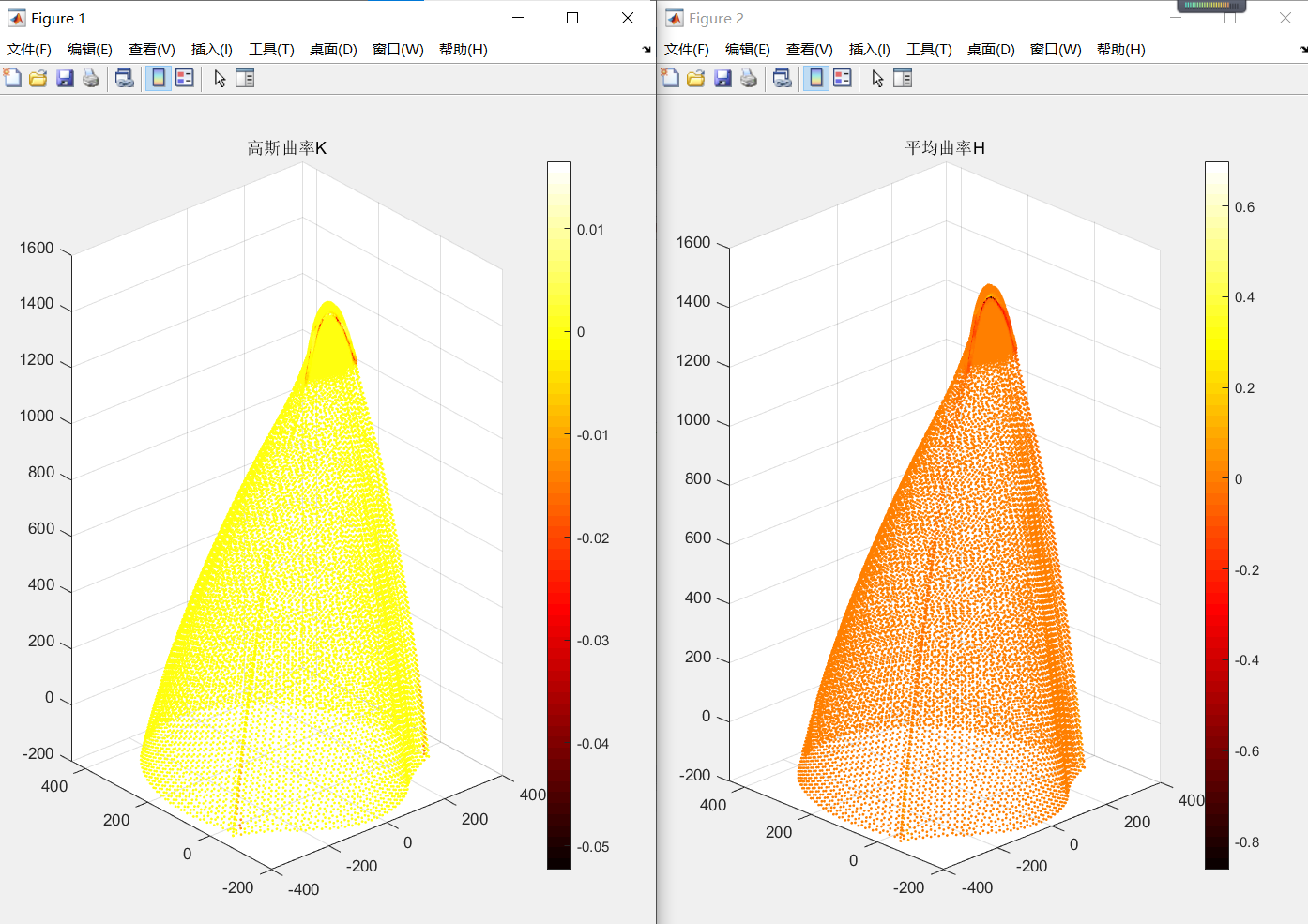

欧氏距离

ESF

ISS算法（Intrinsic shape signatures，内部形状描述子）

算法原理：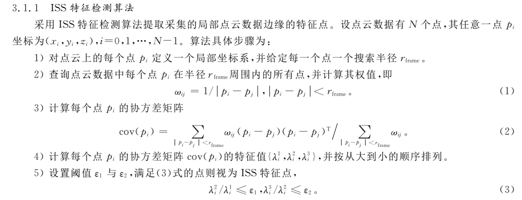

算法实现：

clc
clear
close all
% P = ascread('bun000.asc');
% P = P{2};
% figure;
% x=P(1,1:1:end);
% y=P(2,(1:1:end));
% z=P(3,(1:1:end));
ptCloud=pcread('SR_58_1.pcd');
x=ptCloud.Location(:,1);
y=ptCloud.Location(:,2);
z=ptCloud.Location(:,3);
P=[x';y';z'];
c=z+1;
scatter3(x,y,z,1,c,'filled');
colorbar
view(2)
title('原始数据')
Mdl_p = createns(P','NSMethod','kdtree','Distance','minkowski','p',2);
% [idx_rn_p,dis_p]=rangesearch(Mdl_p,P',0.005);
% idx_fe_p = My_ISS(P,0.005,0.8,0.4,idx_rn_p,dis_p);
[idx_rn_p,dis_p]=rangesearch(Mdl_p,P',50);
idx_fe_p = My_ISS(P,50,0.8,0.4,idx_rn_p,dis_p);

figure;
x=P(1,idx_fe_p(1:1:end));
y=P(2,idx_fe_p(1:1:end));
z=P(3,idx_fe_p(1:1:end));
c=z+1;

scatter3(x,y,z,2,c,'filled');
colorbar
view(2)
title('关键点选取结果')

% (P：点云数据；r：邻域半径；e1,e2:特征值阈值)
function idx_feature = My_ISS(p, r, e1,e2,idx,dis)
if nargin < 4
    error('no bandwidth specified')
end
if nargin < 5
    Mdl = createns(p','NSMethod','kdtree','Distance','minkowski','p',2);
    [idx,dis] = rangesearch(Mdl,p',r);
end
numpts = size(p,2);
flag = zeros(1,numpts);
% tzz = zeros(size(p));
for i = 1:numpts
    if length(idx{i})<2
        continue
    end
    x = p(:,idx{i}(2:end));%r邻域点坐标
    w = 1./dis{i}(2:end);
    p_bar = p(:,i);% 中心点坐标
    P = repmat(w,3,1).*(x - repmat(p_bar,1,size(x,2))) * ...
        transpose(x - repmat(p_bar,1,size(x,2))); %spd matrix P
    P = P./sum(w);
%     if any(isnan(P(:)))
%         save debug.mat 
%     end
    [~,D] = eig(P);
    lam = sort(abs(diag(D)),'descend');% 三个特征值由大到小排列
    if lam(2)/lam(1)<=e1 &&lam(3)/lam(2)<e2
        flag(i)=1;
    end
%     tzz(:,i)=lam;
end
% tzz(1,:)=tzz(2,:)./tzz(1,:);
% tzz(2,:)=tzz(3,:)./tzz(2,:);
% tzz(3,:)=[];
idx_feature = find(flag);
end

实现结果：
调节近邻半径和阈值e1和e2，特征点的稀疏程度也会有所不同，可见模型的棱边会被清晰的提取出来，但是头部区域还是比较混乱。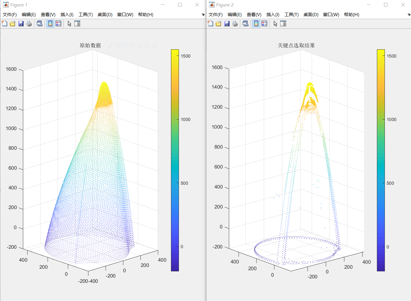

SHOT

FPFH

step4:点云分割

通过参考资料、学术文献检索、阅读，终于确定了待处理问题的专业术语——点云分割，其作用在于将按照一定的规则将点云划分为很多区域，便于后续单独处理。

常用的点云模型分割算法主要包括基于边缘的分割算法、基于区域的分割算法、基于聚类的分割算法以及混合分割算法。

参考文献：
点云模型分割与融合关键技术研究_孙金虎.pdf
Detection of closed sharp edges in point clouds using normal estimation and graph theory.pdf
基于曲率特征的点云数据区域分割和钣金件曲面拟合的技术研究_李海伦.pdf
基于超体素区域增长的点云分割算法研究_姜媛媛.pdf
基于几何特征的三维点云分割算法研究_侯琳琳.pdf
基于局部表面凸性的散乱点云分割算法研究_王雅男.pdf
基于区域增长方法的点云分割算法及环境搭建_介维.pdf
三维点云数据预处和分割算法的研究_刘阳阳.pdf
FCM算法（模糊C均值聚类算法）
算法原理

step5:点云融合

将不同的点云区域拼接起来这一过程的专业表述为：点云融合。我们可以基于融合算法来生成交界面处的过渡。

番外（编程学习）

PCL点云库和VS2019安装