数据表转换
R版本与运行环境信息
Date:2021-4-14R version 4.0.3 (2020-10-10)Platform: x86_64-w64-mingw32/x64 (64-bit)Running under: Windows 10 x64 (build 18363)
载入相关包
library(tidyverse)setwd("G:\\Desktop\\s_note\\data\\data2clean")df <- read.csv("df.csv")
数据查看
- 查看数据
> dfID A1 A2 A3 A4 A5 A6 A7 A8 A9 A101 T_1 1.866507 3.038351 2.779211 1.606315 1.001641 8.577044 4.683432 5.163498 3.231970 5.6351332 T_2 4.445010 2.721566 4.797077 6.861528 1.272664 5.840218 8.330187 3.248087 6.423117 9.5271563 T_3 7.077780 8.095160 1.826613 2.737936 5.897779 5.017294 5.729174 6.960172 8.999864 2.4378484 T_4 3.719282 4.840970 8.024423 8.301709 5.664989 8.680034 2.702984 7.555995 1.997212 6.5080565 T_5 2.661250 8.839854 4.805376 2.711006 9.752574 3.498883 6.594125 9.650040 5.391911 5.7923266 T_6 2.056874 8.421298 1.580424 2.796107 9.757730 4.045160 2.756127 5.573386 2.222584 9.0351457 T_7 5.873148 7.886457 5.646370 3.603152 1.399365 1.826301 2.891329 5.860019 9.476443 6.4088618 T_8 9.458056 3.692235 2.429818 2.433509 8.162586 5.246516 7.630174 1.654225 9.279964 6.6215709 T_9 9.765868 4.460042 8.002026 4.315732 6.215334 3.019176 6.437253 5.999071 3.435929 9.13448410 T_10 1.328430 7.676231 2.743958 5.028596 7.816146 7.840817 2.674568 9.824781 2.804552 3.707074
> df2ID ID2 A1 A2 A3 A4 A5 A6 A7 A8 A9 A101 T_1 T1 1.866507 3.038351 2.779211 1.606315 1.001641 8.577044 4.683432 5.163498 3.231970 5.6351332 T_2 T1 4.445010 2.721566 4.797077 6.861528 1.272664 5.840218 8.330187 3.248087 6.423117 9.5271563 T_3 T1 7.077780 8.095160 1.826613 2.737936 5.897779 5.017294 5.729174 6.960172 8.999864 2.4378484 T_4 R2 3.719282 4.840970 8.024423 8.301709 5.664989 8.680034 2.702984 7.555995 1.997212 6.5080565 T_5 R2 2.661250 8.839854 4.805376 2.711006 9.752574 3.498883 6.594125 9.650040 5.391911 5.7923266 T_6 R2 2.056874 8.421298 1.580424 2.796107 9.757730 4.045160 2.756127 5.573386 2.222584 9.0351457 T_7 T3 5.873148 7.886457 5.646370 3.603152 1.399365 1.826301 2.891329 5.860019 9.476443 6.4088618 T_8 T3 9.458056 3.692235 2.429818 2.433509 8.162586 5.246516 7.630174 1.654225 9.279964 6.6215709 T_9 T3 9.765868 4.460042 8.002026 4.315732 6.215334 3.019176 6.437253 5.999071 3.435929 9.13448410 T_10 T3 1.328430 7.676231 2.743958 5.028596 7.816146 7.840817 2.674568 9.824781 2.804552 3.707074
宽数据—>长数据
**gather**: 宽数据转换为长数据
**key**: 宽数据的列名转换成长数据后对应列的列名**value**: 转换后,值所对应列的列名...: 指定哪列用于转换,使用**-**(减号),则代表除了某一列外所有的数据进行转换, 一般会将因子所在的列去掉(-因子)**factor_key**: 默认FALSE,转换后的数据按照字符串的顺序排列,TURE则按照原顺序排列
#宽数据-->长数据df.long <- gather(data = df,key = Index,value = a_value,-ID)#df.long <- gather(data = df,key = Index,value = a_value,A1:A10,factor_key = T)head(df.long)> head(df.long)ID Index a_value1 T_1 A1 1.8665072 T_2 A1 4.4450103 T_3 A1 7.0777804 T_4 A1 3.7192825 T_5 A1 2.6612506 T_6 A1 2.056874#存在多列分组时df2 <- read.csv("df2.csv")df2.long <- gather(data = df2,key = Index,value = a_value,-c(ID,ID2))#df2.long <- gather(data = df2,key = Index,value = a_value,A1:A10,factor_key = T)head(df2.long)ID ID2 Index a_value1 T_1 T1 A1 1.8665072 T_2 T1 A1 4.4450103 T_3 T1 A1 7.0777804 T_4 R2 A1 3.7192825 T_5 R2 A1 2.6612506 T_6 R2 A1 2.056874
长数据—>宽数据
**spread** :长数据转换为宽数据
**key**: 指定列名,该列转换后为宽数据的列名**value**: 指定数据所在列的列名**fill**: 如果存在缺失值则使用fill指定的值进行填充**convert**: 可以识别某列的数据类型,并自动转换,通常用于转换后的列中有多种数据类型,可以即根据不同的数据类型进行转换, 如value所在列既有字符串也有数值(This is useful if the value column was a mix of variables that was coerced to a string)
#长数据-->宽数据df.wid <- spread(data = df.long,key = Index,value = a_value)df.wid> df.widID A2 A3 A4 A5 A6 A7 A8 A9 A10 A11 T_1 3.038351 2.779211 1.606315 1.001641 8.577044 4.683432 5.163498 3.231970 5.635133 1.8665072 T_2 2.721566 4.797077 6.861528 1.272664 5.840218 8.330187 3.248087 6.423117 9.527156 4.4450103 T_3 8.095160 1.826613 2.737936 5.897779 5.017294 5.729174 6.960172 8.999864 2.437848 7.0777804 T_4 4.840970 8.024423 8.301709 5.664989 8.680034 2.702984 7.555995 1.997212 6.508056 3.7192825 T_5 8.839854 4.805376 2.711006 9.752574 3.498883 6.594125 9.650040 5.391911 5.792326 2.6612506 T_6 8.421298 1.580424 2.796107 9.757730 4.045160 2.756127 5.573386 2.222584 9.035145 2.0568747 T_7 7.886457 5.646370 3.603152 1.399365 1.826301 2.891329 5.860019 9.476443 6.408861 5.8731488 T_8 3.692235 2.429818 2.433509 8.162586 5.246516 7.630174 1.654225 9.279964 6.621570 9.4580569 T_9 4.460042 8.002026 4.315732 6.215334 3.019176 6.437253 5.999071 3.435929 9.134484 9.76586810 T_10 7.676231 2.743958 5.028596 7.816146 7.840817 2.674568 9.824781 2.804552 3.707074 1.328430df2.wid <- spread(data = df2.long,key = Index,value = a_value,convert = T)df2.widID ID2 A1 A10 A2 A3 A4 A5 A6 A7 A8 A91 T_1 T1 1.866507 5.635133 3.038351 2.779211 1.606315 1.001641 8.577044 4.683432 5.163498 3.2319702 T_10 T3 1.328430 3.707074 7.676231 2.743958 5.028596 7.816146 7.840817 2.674568 9.824781 2.8045523 T_2 T1 4.445010 9.527156 2.721566 4.797077 6.861528 1.272664 5.840218 8.330187 3.248087 6.4231174 T_3 T1 7.077780 2.437848 8.095160 1.826613 2.737936 5.897779 5.017294 5.729174 6.960172 8.9998645 T_4 R2 3.719282 6.508056 4.840970 8.024423 8.301709 5.664989 8.680034 2.702984 7.555995 1.9972126 T_5 R2 2.661250 5.792326 8.839854 4.805376 2.711006 9.752574 3.498883 6.594125 9.650040 5.3919117 T_6 R2 2.056874 9.035145 8.421298 1.580424 2.796107 9.757730 4.045160 2.756127 5.573386 2.2225848 T_7 T3 5.873148 6.408861 7.886457 5.646370 3.603152 1.399365 1.826301 2.891329 5.860019 9.4764439 T_8 T3 9.458056 6.621570 3.692235 2.429818 2.433509 8.162586 5.246516 7.630174 1.654225 9.27996410 T_9 T3 9.765868 9.134484 4.460042 8.002026 4.315732 6.215334 3.019176 6.437253 5.999071 3.435929
数据分割
**separate** :数据分割,指定分割符或按照长度进行分割
**data**: 指定数据**col**: 指定要分割的列**into**: 指定要分成几列,以及每列的名字,正常是等于分割完的列数,指定的列数如果小于或大于分割后的列数应该使用extra或fill进行调整**sep**: 指定分割符,可以是符号或index,同时支持-index**fill**: 当分割后的列数多于into的列数时候,指定NA值的位置,left/right/warn(默认)左侧/右侧/右侧且不忽略警告信息;**extra**: 当分割后的列数少于into的列数时候,指定多余列的处理方式,drop/merge/warn(默认)-丢掉/与第二列合并/丢掉且不忽略警告信息;**remove**: 是否保留分割前的数据列,默认FALSE**convert**: 同上
df3 <- data.frame(df2,ID3=str_c(df2$ID,"_",df2$ID2 )) %>% select(ID3,str_c("A",c(1:10)))#数据分割separate(data = df3,col = ID3,into = c("A","b","c"),sep = "_")separate(data = df3,col = ID3,into = c("A","b"),sep = -3,extra = "merge")separate(data = df3,col = ID3,into = c("A","b"),sep = "_",extra = "merge")
行列匹配与行列排序
#构建示例数据df <- tibble(grammer=c("Python","C","Java","Go",NA,"SQL","PHP","Python","Python"),score=c("1","2",NA,"4","5","6","7","10","15"))> df# A tibble: 9 x 2grammer score<chr> <chr>1 Python 12 C 23 Java NA4 Go 45 NA 56 SQL 67 PHP 78 Python 109 Python 15
**str_detect**:进行数据的条件提取,提取包含某字符的列/行, 支持正则,详见stringr学习,可以替代grep
df[str_detect(df$grammer,string = "Python"),]#输出结果> df[str_detect(df$grammer,string = "Python"),]# A tibble: 4 x 2grammer score<chr> <chr>1 Python 12 NA NA3 Python 104 Python 15
**filter**: 按行筛选, 支持字符与数字,使用==进行比较时,比较浮点数的大小时应该使用**near()**函数进行比较,用法如下
使用between()函数代替score >= 2 & score < 5.0, >>between(score,2,5)
df %>% filter(grammer == "Python")#使用%in%可以让代码更加简洁和可读,避免使用多个 |df %>% filter(grammer %in% c("Python","c","Java"))df %>% filter(score == 10)df %>% filter(score >= 2)df %>% filter(score >= 2 & score < 5.0)df %>% filter(score >= 2 | score < 5.0)df %>% filter(score != 2 )###near函数的使用#使用==时,由于浮点数和int的问题使结果有问题> sqrt(2) ^2 == 2[1] FALSE#使用near函数进行比较> near(sqrt(2)^2,2)[1] TRUE
**select**: 按列筛选,可以筛选包含某字段的列,同时可以配合一些辅助函数进行使用,如contains(): 筛选包含某字符的列starts_with(): 筛选以指定字符开头的列ends_with: 筛选以指定字符结尾的列matches(): 使用正则表达式筛选everything(): 配合这一函数使用,可以将select函数所选中的列排在前面,后面列顺序保持不变
df %>% select(score)#使用此方法可以对列进行重新排序df %>% select(c(score,grammer))> df %>% select(c(score,grammer))# A tibble: 9 x 2score grammer<chr> <chr>1 1 Python2 2 C3 NA Java4 4 Go......#配合contains函数实现筛选包含某一字段的列df %>% select(contains("s"))> df %>% select(contains("s"))# A tibble: 9 x 1score<chr>1 12 23 NA4 4......
缺失值的处理
使用is.na()判断是否存在缺失值,结合filter()函数可以实现对含有NA行的筛选,同时结合! (取反)可以实现筛选不含NA的行
#以nycflights13的数据为例子library(tidyverse)library(nycflights13)#dep_time包含缺失值的行#使用基础函数flights[is.na(flights$dep_time),]> flights[is.na(flights$dep_time),1:5]# A tibble: 8,255 x 5year month day dep_time sched_dep_time<int> <int> <int> <int> <int>1 2013 1 1 NA 16302 2013 1 1 NA 19353 2013 1 1 NA 15004 2013 1 1 NA 6005 2013 1 2 NA 1540......#使用filterflights %>% filter(is.na(flights$dep_time)) %>% select(1:5)# A tibble: 8,255 x 5year month day dep_time sched_dep_time<int> <int> <int> <int> <int>1 2013 1 1 NA 16302 2013 1 1 NA 19353 2013 1 1 NA 15004 2013 1 1 NA 6005 2013 1 2 NA 1540
使用mutate增加新的一列
使用mutate可以新增加一列,该列必须和表格中的行数相等,否则报错,同时使用transmute()可以实现仅仅保留增加的列
#继续以flights数据为例子#首先选择flights中的year,以及dest到hour列,使用了mutate增加了两列df <-flights %>% select(year,dest:hour) %>% mutate(speed = distance / hour,other = air_time + hour)> df# A tibble: 336,776 x 7year dest air_time distance hour speed other<int> <chr> <dbl> <dbl> <dbl> <dbl> <dbl>1 2013 IAH 227 1400 5 280 2322 2013 IAH 227 1416 5 283. 2323 2013 MIA 160 1089 5 218. 1654 2013 BQN 183 1576 5 315. 188......# ... with 336,766 more rows#使用transmute则可以仅仅保留添加的列df <-flights %>% select(year,dest:hour) %>% transmute(speed = distance / hour,other = air_time + hour)> df# A tibble: 336,776 x 2speed other<dbl> <dbl>1 280 2322 283. 2323 218. 165......# ... with 336,766 more rows
数据的组合
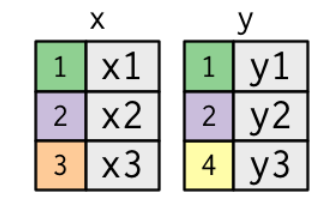
给定两个数据集,x和y
使用**inner_join**,**left_join**, **right_join**, **full_join**等函数对数据表进行组合,基本流程就成,需要全部保留的数据将**by =**选项指定的全部数据留下,另一个数据框开始匹配,如果可以匹配上则填入相应数据,反之则填入**NA**
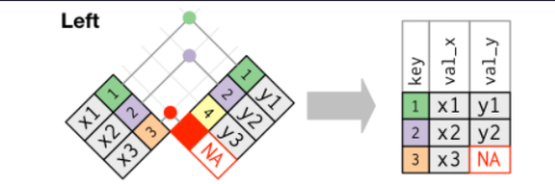
**left_join**:左连接,保留左侧(x)的全部数据,左侧为准
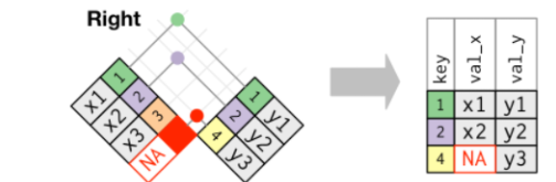
**right_join**: 右连接,保留右侧(y)的全部数据。右侧为准
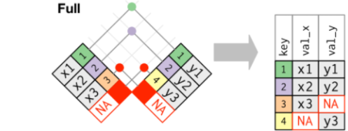
**full_join**: 全连接,保留所有的数据
**inner_join**: 仅仅找共有的数据
数据的行名不存在一对多的情况
#构建测试数据library(tidyverse)df.x <- tibble(name = c(1,2,3),> df.x# A tibble: 3 x 2name value_x<dbl> <chr>1 1 x12 2 x23 3 x3df.y <- tibble(name = c(1,2,4,5),value_y = c("y1","y2","y3","y4"))> df.y# A tibble: 4 x 2name value_y<dbl> <chr>1 1 y12 2 y23 4 y34 5 y4#——————左连接——————#保留了x的所有name,y数据并没有name = 3对应的值,所以为NAdf.x %>% left_join(df.y,by = "name")# A tibble: 3 x 3name value_x value_y<dbl> <chr> <chr>1 1 x1 y12 2 x2 y23 3 x3 NA#——————右连接——————df.x %>% right_join(df.y,by = "name")# A tibble: 4 x 3name value_x value_y<dbl> <chr> <chr>1 1 x1 y12 2 x2 y23 4 NA y34 5 NA y4#保留y的names,同时names=4 5的时候x没有对应值,所以为NA#——————内连接——————df.x %>% inner_join(df.y,by = "name")# A tibble: 2 x 3name value_x value_y<dbl> <chr> <chr>1 1 x1 y12 2 x2 y2#仅仅取了两个数据集共有的部分#——————全连接——————df.x %>% full_join(df.y,by = "name")# A tibble: 5 x 3name value_x value_y<dbl> <chr> <chr>1 1 x1 y12 2 x2 y23 3 x3 NA4 4 NA y35 5 NA y4#names所有值都保留

若有收获,就点个赞吧
0 人点赞
