4. 聚合分析
4.1. bucket
4.2. metric
metric是对一个bucket执行的某种聚合分析操作。 count avg max min sum 等操作。示例
建索引tvs
PUT /tvs{"mappings": {"properties": {"price": {"type": "long"},"color": {"type": "keyword"},"brand": {"type": "keyword"},"sold_date": {"type": "date"}}}}
测试数据
POST /tvs/_bulk
{
  "index": {}
}
{
"price": 1000,
"color": "红色",
"brand": "长虹",
"sold_date": "2016-10-28"
}
{
  "index": {}
}
{
"price": 2000,
"color": "红色",
"brand": "长虹",
"sold_date": "2016-11-05"
}
{
  "index": {}
}
{
  "price": 3000,
  "color": "绿色",
  "brand": "小米",
  "sold_date": "2016-05-18"
}
{
  "index": {}
}
{
"price": 1500,
"color": "蓝色",
"brand": "TCL",
"sold_date": "2016-07-02"
}
{
  "index": {}
}
{
"price": 1200,
"color": "绿色",
"brand": "TCL",
"sold_date": "2016-08-19"
}
{
  "index": {}
}
{
"price": 2000,
"color": "红色",
"brand": "长虹",
"sold_date": "2016-11-05"
}
{
  "index": {}
}
{
"price": 8000,
"color": "红色",
"brand": "三星",
"sold_date": "2017-01-01"
}
{
  "index": {}
}
{
"price": 2500,
"color": "蓝色",
"brand": "小米",
"sold_date": "2017-02-12"
}
4.2.1. 按数量分组
统计某种颜色电视机销量最高
GET /tvs/_search
{
  "size" : 0,
  "aggs" : {
      "popular_colors" : {
          "terms" : {
            "field" : "color"
          }
      }
  }
}
请求参数含义:
size:只获取聚合结果,而不需要返回执行聚合的那些原始数据;
- aggs:固定语法,表示要对一份数据执行分组聚合操作;
- popular_colors:每个aggs的名字,自定义;
- terms:根据字段值进行分组;
- field:进行分组的字段。
返回结果:
{
  "took" : 7,
  "timed_out" : false,
  "_shards" : {
    "total" : 1,
    "successful" : 1,
    "skipped" : 0,
    "failed" : 0
  },
  "hits" : {
    "total" : {
      "value" : 8,
      "relation" : "eq"
    },
    "max_score" : null,
    "hits" : [ ]
  },
  "aggregations" : {
    "popular_colors" : {
      "doc_count_error_upper_bound" : 0,
      "sum_other_doc_count" : 0,
      "buckets" : [
        {
          "key" : "红色",
          "doc_count" : 4
        },
        {
          "key" : "绿色",
          "doc_count" : 2
        },
        {
          "key" : "蓝色",
          "doc_count" : 2
        }
      ]
    }
  }
}
出参含义:
hits.hits我们在请求中指定了size=0,所以hits.hits就是空的,否则会把执行聚合的那些原始数据返回。aggregations聚合结果。popular_color自定义的聚合名称。buckets根据我们指定的field划分出的 buckets。keyfield的值。doc_count这个 bucket 分组内的 doc 条数。按数量分组其实并不算是一个metric操作,它是Elasticsearch对聚合分析的一种默认操作,利用term实现。
4.2.2. 统计平均值
统计每种颜色电视机的平均价格:
GET /tvs/_search
{
   "size" : 0,
   "aggs": {
      "colors": {
         "terms": {
            "field": "color"
         },
         "aggs": {
            "avg_price": {
               "avg": {
                  "field": "price"
               }
            }
         }
      }
   }
}
嵌套 aggs 与 terms 平级,对每个bucket执行一次metric操作。
返回结果:
{
  "took" : 12,
  "timed_out" : false,
  "_shards" : {
    "total" : 1,
    "successful" : 1,
    "skipped" : 0,
    "failed" : 0
  },
  "hits" : {
    "total" : {
      "value" : 8,
      "relation" : "eq"
    },
    "max_score" : null,
    "hits" : [ ]
  },
  "aggregations" : {
    "colors" : {
      "doc_count_error_upper_bound" : 0,
      "sum_other_doc_count" : 0,
      "buckets" : [
        {
          "key" : "红色",
          "doc_count" : 4,
          "avg_price" : {
            "value" : 3250.0
          }
        },
        {
          "key" : "绿色",
          "doc_count" : 2,
          "avg_price" : {
            "value" : 2100.0
          }
        },
        {
          "key" : "蓝色",
          "doc_count" : 2,
          "avg_price" : {
            "value" : 2000.0
          }
        }
      ]
    }
  }
}
avg_price 的 value 为 metric 计算的结果,每个 bucket 中的所有 doc 的 price 字段值的平均值。
4.2.3. 下钻分析
对bucket再分组,再对每个最小粒度分组执行聚合分析操作。例如:按照颜色对电视机进行分组,再对每种颜色下的各个品牌电视机求平均价格:
GET /tvs/_search
{
  "size": 0,
  "aggs": {
    "group_by_color": {
      "terms": {
        "field": "color"
      },
      "aggs": {
        "color_avg_price": {
          "avg": {
            "field": "price"
          }
        },
        "group_by_brand": {
          "terms": {
            "field": "brand"
          },
          "aggs": {
            "brand_avg_price": {
              "avg": {
                "field": "price"
              }
            }
          }
        }
      }
    }
  }
}
嵌套 group_by_brand 按照band字段进行分组,求品牌的平均价格。
返回结果:
{
  "took" : 54,
  "timed_out" : false,
  "_shards" : {
    "total" : 1,
    "successful" : 1,
    "skipped" : 0,
    "failed" : 0
  },
  "hits" : {
    "total" : {
      "value" : 8,
      "relation" : "eq"
    },
    "max_score" : null,
    "hits" : [ ]
  },
  "aggregations" : {
    "group_by_color" : {
      "doc_count_error_upper_bound" : 0,
      "sum_other_doc_count" : 0,
      "buckets" : [
        {
          "key" : "红色",
          "doc_count" : 4,
          "color_avg_price" : {
            "value" : 3250.0
          },
          "group_by_brand" : {
            "doc_count_error_upper_bound" : 0,
            "sum_other_doc_count" : 0,
            "buckets" : [
              {
                "key" : "长虹",
                "doc_count" : 3,
                "brand_avg_price" : {
                  "value" : 1666.6666666666667
                }
              },
              {
                "key" : "三星",
                "doc_count" : 1,
                "brand_avg_price" : {
                  "value" : 8000.0
                }
              }
            ]
          }
        },
        {
          "key" : "绿色",
          "doc_count" : 2,
          "color_avg_price" : {
            "value" : 2100.0
          },
          "group_by_brand" : {
            "doc_count_error_upper_bound" : 0,
            "sum_other_doc_count" : 0,
            "buckets" : [
              {
                "key" : "TCL",
                "doc_count" : 1,
                "brand_avg_price" : {
                  "value" : 1200.0
                }
              },
              {
                "key" : "小米",
                "doc_count" : 1,
                "brand_avg_price" : {
                  "value" : 3000.0
                }
              }
            ]
          }
        },
        {
          "key" : "蓝色",
          "doc_count" : 2,
          "color_avg_price" : {
            "value" : 2000.0
          },
          "group_by_brand" : {
            "doc_count_error_upper_bound" : 0,
            "sum_other_doc_count" : 0,
            "buckets" : [
              {
                "key" : "TCL",
                "doc_count" : 1,
                "brand_avg_price" : {
                  "value" : 1500.0
                }
              },
              {
                "key" : "小米",
                "doc_count" : 1,
                "brand_avg_price" : {
                  "value" : 2500.0
                }
              }
            ]
          }
        }
      ]
    }
  }
}
4.2.4. 统计极值
统计每种颜色的电视机的最高价和最低价:
GET /tvs/_search
{
   "size" : 0,
   "aggs": {
      "colors": {
         "terms": {
            "field": "color"
         },
         "aggs": {
            "min_price" : { "min": { "field": "price"} },
            "max_price" : { "max": { "field": "price"} }
         }
      }
   }
}
4.3. histogram
histogram关键字来完成对指定字段值的 区间分组 ,如果我们想要分组的字段类型为日期,则需要使用 date_histogram 关键字。
接收一个field,按照field值的各个范围区间,进行bucket分组操作:
GET /tvs/_search
{
 "size" : 0,
 "aggs":{
    "price":{
       "histogram":{
          "field": "price",
          "interval": 2000
       }
    }
 }
}
上述请求中,我们对“price”字段进行区间分组,区间间隔为2000,返回结果:
{
"took" : 3,
"timed_out" : false,
"_shards" : {
  "total" : 1,
  "successful" : 1,
  "skipped" : 0,
  "failed" : 0
},
"hits" : {
  "total" : {
    "value" : 8,
    "relation" : "eq"
  },
  "max_score" : null,
  "hits" : [ ]
},
"aggregations" : {
  "price" : {
    "buckets" : [
      {
        "key" : 0.0,
        "doc_count" : 3
      },
      {
        "key" : 2000.0,
        "doc_count" : 4
      },
      {
        "key" : 4000.0,
        "doc_count" : 0
      },
      {
        "key" : 6000.0,
        "doc_count" : 0
      },
      {
        "key" : 8000.0,
        "doc_count" : 1
      }
    ]
  }
}
}
按照区间分组之后,我们就可以对各个 bucket 执行 metric 操作了,比如计算总和:
GET /tvs/_search
{
 "size" : 0,
 "aggs":{
    "price":{
       "histogram":{
          "field": "price",
          "interval": 2000
       },
       "aggs":{
          "revenue": {
             "sum": {
               "field" : "price"
             }
           }
       }
    }
 }
}
4.3.1. date_histogram
按区间分组的字段是 date 类型,需要用到 date_histogram 关键字,例如:
GET /tvs/_search
{
 "size" : 0,
 "aggs": {
    "sales": {
       "date_histogram": {
          "field": "sold_date",
          "interval": "month",
          "format": "yyyy-MM-dd",
          "min_doc_count" : 0,
          "extended_bounds" : {
              "min" : "2016-01-01",
              "max" : "2017-12-31"
          }
       }
    }
 }
}
入参说明:
min_doc_count某个日期区间内的doc数量至少要等于这个参数,这个区间才会返回。extended_bounds划分bucket的时候,会限定在这个起始日期和截止日期内。
统计每季度每个品牌的电视销售额:
GET /tvs/_search
{
  "size": 0,
  "aggs": {
    "group_by_sold_date": {
      "date_histogram": {
        "field": "sold_date",
        "interval": "quarter",
        "format": "yyyy-MM-dd",
        "min_doc_count": 0,
        "extended_bounds": {
          "min": "2016-01-01",
          "max": "2017-12-31"
        }
      },
      "aggs": {
        "total_sum_price": {
          "sum": {
            "field": "price"
          }
        },
        "group_by_brand": {
          "terms": {
            "field": "brand"
          },
          "aggs": {
            "sum_price": {
              "sum": {
                "field": "price"
              }
            }
          }
        }
      }
    }
  }
}
先按日期进行分组,然后下钻到组内再按照品牌分组,最后对每个子组执行求和metric操作。结果如下:
{
  "took" : 97,
  "timed_out" : false,
  "_shards" : {
    "total" : 1,
    "successful" : 1,
    "skipped" : 0,
    "failed" : 0
  },
  "hits" : {
    "total" : {
      "value" : 8,
      "relation" : "eq"
    },
    "max_score" : null,
    "hits" : [ ]
  },
  "aggregations" : {
    "group_by_sold_date" : {
      "buckets" : [
        {
          "key_as_string" : "2016-01-01",
          "key" : 1451606400000,
          "doc_count" : 0,
          "total_sum_price" : {
            "value" : 0.0
          },
          "group_by_brand" : {
            "doc_count_error_upper_bound" : 0,
            "sum_other_doc_count" : 0,
            "buckets" : [ ]
          }
        },
        {
          "key_as_string" : "2016-04-01",
          "key" : 1459468800000,
          "doc_count" : 1,
          "total_sum_price" : {
            "value" : 3000.0
          },
          "group_by_brand" : {
            "doc_count_error_upper_bound" : 0,
            "sum_other_doc_count" : 0,
            "buckets" : [
              {
                "key" : "小米",
                "doc_count" : 1,
                "sum_price" : {
                  "value" : 3000.0
                }
              }
            ]
          }
        },
        {
          "key_as_string" : "2016-07-01",
          "key" : 1467331200000,
          "doc_count" : 2,
          "total_sum_price" : {
            "value" : 2700.0
          },
          "group_by_brand" : {
            "doc_count_error_upper_bound" : 0,
            "sum_other_doc_count" : 0,
            "buckets" : [
              {
                "key" : "TCL",
                "doc_count" : 2,
                "sum_price" : {
                  "value" : 2700.0
                }
              }
            ]
          }
        },
        {
          "key_as_string" : "2016-10-01",
          "key" : 1475280000000,
          "doc_count" : 3,
          "total_sum_price" : {
            "value" : 5000.0
          },
          "group_by_brand" : {
            "doc_count_error_upper_bound" : 0,
            "sum_other_doc_count" : 0,
            "buckets" : [
              {
                "key" : "长虹",
                "doc_count" : 3,
                "sum_price" : {
                  "value" : 5000.0
                }
              }
            ]
          }
        },
        {
          "key_as_string" : "2017-01-01",
          "key" : 1483228800000,
          "doc_count" : 2,
          "total_sum_price" : {
            "value" : 10500.0
          },
          "group_by_brand" : {
            "doc_count_error_upper_bound" : 0,
            "sum_other_doc_count" : 0,
            "buckets" : [
              {
                "key" : "三星",
                "doc_count" : 1,
                "sum_price" : {
                  "value" : 8000.0
                }
              },
              {
                "key" : "小米",
                "doc_count" : 1,
                "sum_price" : {
                  "value" : 2500.0
                }
              }
            ]
          }
        },
        {
          "key_as_string" : "2017-04-01",
          "key" : 1491004800000,
          "doc_count" : 0,
          "total_sum_price" : {
            "value" : 0.0
          },
          "group_by_brand" : {
            "doc_count_error_upper_bound" : 0,
            "sum_other_doc_count" : 0,
            "buckets" : [ ]
          }
        },
        {
          "key_as_string" : "2017-07-01",
          "key" : 1498867200000,
          "doc_count" : 0,
          "total_sum_price" : {
            "value" : 0.0
          },
          "group_by_brand" : {
            "doc_count_error_upper_bound" : 0,
            "sum_other_doc_count" : 0,
            "buckets" : [ ]
          }
        },
        {
          "key_as_string" : "2017-10-01",
          "key" : 1506816000000,
          "doc_count" : 0,
          "total_sum_price" : {
            "value" : 0.0
          },
          "group_by_brand" : {
            "doc_count_error_upper_bound" : 0,
            "sum_other_doc_count" : 0,
            "buckets" : [ ]
          }
        }
      ]
    }
  }
}
4.4. Aggregation Scope
限定进行聚合分析的doc范围,可以和query、filter结合使用。**聚合分析与全文检索结合使用**
Elasticsearch中的所有聚合都会在一个scope下执行,结合普通搜索请求后,这个scope就是检索出的结果。
例如:统计指定品牌下每个颜色的销量:
GET /tvs/_search
{
  "size": 0,
  "query": {
    "term": {
      "brand": {
        "value": "小米"
      }
    }
  },
  "aggs": {
    "group_by_color": {
      "terms": {
        "field": "color"
      }
    }
  }
}
结果:
{
  "took" : 34,
  "timed_out" : false,
  "_shards" : {
    "total" : 1,
    "successful" : 1,
    "skipped" : 0,
    "failed" : 0
  },
  "hits" : {
    "total" : {
      "value" : 2,
      "relation" : "eq"
    },
    "max_score" : null,
    "hits" : [ ]
  },
  "aggregations" : {
    "group_by_color" : {
      "doc_count_error_upper_bound" : 0,
      "sum_other_doc_count" : 0,
      "buckets" : [
        {
          "key" : "绿色",
          "doc_count" : 1
        },
        {
          "key" : "蓝色",
          "doc_count" : 1
        }
      ]
    }
  }
}
**聚合分析与filter结合使用** 例如:下面的请求是统计价格大于1200的所有电视机的平均价格。
GET /tvs/_search
{
  "size": 0,
  "query": {
    "constant_score": {
      "filter": {
        "range": {
          "price": {
            "gte": 1200
          }
        }
      }
    }
  },
  "aggs": {
    "avg_price": {
      "avg": {
        "field": "price"
      }
    }
  }
}
针对某个bucket进行精细化的filter,那么就可以使用aggs.filter。例如:统计长虹电视最近1个月、最近3个月、最近6个月的平均值:
GET /tvs/_search
{
  "size": 0,
  "query": {
    "term": {
      "brand": {
        "value": "长虹"
      }
    }
  },
  "aggs": {
    "recent_1m": {
      "filter": {
        "range": {
          "sold_date": {
            "gte": "now-1m"
          }
        }
      },
      "aggs": {
        "recent_1m_avg_price": {
          "avg": {
            "field": "price"
          }
        }
      }
    },
    "recent_3m": {
      "filter": {
        "range": {
          "sold_date": {
            "gte": "now-3m"
          }
        }
      },
      "aggs": {
        "recent_3m_avg_price": {
          "avg": {
            "field": "price"
          }
        }
      }
    },
    "recent_6m": {
      "filter": {
        "range": {
          "sold_date": {
            "gte": "now-6m"
          }
        }
      },
      "aggs": {
        "recent_6m_avg_price": {
          "avg": {
            "field": "price"
          }
        }
      }
    }
  }
}
4.5. global bucket
对于一次聚合分析请求,给出两个结果,对于这种需求使用 global bucket :
- 指定scope范围内的聚合结果;
- 不限定范围的聚合结果。
例如:对比长虹牌电视机的平均销售额和所有品牌电视机的平均销售额:
GET /tvs/_search
{
  "size": 0,
  "query": {
    "term": {
      "brand": {
        "value": "长虹"
      }
    }
  },
  "aggs": {
    "single_brand_avg_price": {
      "avg": {
        "field": "price"
      }
    },
    "all": {
      "global": {},
      "aggs": {
        "all_brand_avg_price": {
          "avg": {
            "field": "price"
          }
        }
      }
    }
  }
}
上述请求中 query 用于限定 scope ,对该 scope 范围内的 doc 执行聚合分析,而内部的 global 关键字会将聚合分析的范围指定为所有 doc 。
请求结果:
{
  "took" : 35,
  "timed_out" : false,
  "_shards" : {
    "total" : 1,
    "successful" : 1,
    "skipped" : 0,
    "failed" : 0
  },
  "hits" : {
    "total" : {
      "value" : 3,
      "relation" : "eq"
    },
    "max_score" : null,
    "hits" : [ ]
  },
  "aggregations" : {
    "all" : {
      "doc_count" : 8,
      "all_brand_avg_price" : {
        "value" : 2650.0
      }
    },
    "single_brand_avg_price" : {
      "value" : 1666.6666666666667
    }
  }
}
一般来讲,有些聚合分析的metric操作,是很容易在多个shard中并行执行的,比如max、min、avg这种,coordinate node拿到各个shard的返回结果后,只需要经过简单计算就能得出最终结果:
- coordinate node把请求广播到所有shard;
- 每个分片计算本地最大的字段值,返回给coordinate node;
- coordinate node选出所有shard返回的最大值,这就是最终的最大值。
上面这类算法可以随着机器数的线性增长而横向扩展,无须任何协调操作(机器之间不需要讨论中间结果),而且内存消耗很小(一个整型就能代表最大值)。
但是还有些算法,是很难并行执行的,比如说count(distinct),并不是说在每个shard上直接过滤出distinct value就可以了,因为coordinate node需要拿到各个shard返回的结果,在内存中进行筛选操作,如果数据量非常大,这个过程非常耗时。
所以,Elasticsearch为了提升性能,采用了近似算法,它们会提供准确但不是 100% 精确的结果, 以牺牲一点小小的估算错误为代价,这些算法可以为我们换来高速的执行效率和极小的内存消耗。
4.6. 近似算法
基本思想就是在 大数据 精确性 实时性 三者之间做出权衡,一般只能选择其中的2个,有点类似于CAP。 因为对于很多应用,能够实时返回高度准确的结果要比 100% 精确结果重要得多:
精确 + 实时
数据可以存入单台机器的内存之中,我们可以随心所欲,使用任何想用的算法。结果会 100% 精确,响应会相对快速。
大数据 + 精确
传统的 Hadoop,可以处理 PB 级的数据并且为我们提供精确的答案,但它可能需要几周的时间才能为我们提供这个答案。
大数据 + 实时
近似算法为我们实时提供准确但不精确的结果。
Elasticsearch 目前支持两种近似算法( cardinality 和 percentiles )。 它们会提供准确但不是 100% 精确的结果,以牺牲一点小小的估算错误为代价,这些算法可以为我们换来高速的执行效率和极小的内存消耗。
4.6.1. Cardinality
用于统计某个字段的不同值的个数,也就是去重统计。例如:统计每个月销售的不同品牌数量:
GET /tvs/_search
{
  "size" : 0,
  "aggs" : {
      "months" : {
        "date_histogram": {
          "field": "sold_date",
          "interval": "month"
        },
        "aggs": {
          "distinct_brand" : {
              "cardinality" : {
                "field" : "brand"
              }
          }
        }
      }
  }
}
算法优化
Cardinality算法的统计结果并不一定精确,但是速度非常快,我们还可以通过调整参数来进一步优化。
- precision_threshold
控制 Cardinality 算法的精确度和内存消耗,它接受 0–40000 之间的数字,更大的值还是会被当作 40000 来处理。
例如: precision_threshold 设置为 100 ,那么Elasticsearch会确保当字段唯一值在 100 以内时,会得到非常准确的结果,这个准确率几乎100%。但是,如果字段唯一值的数目高于precision_threshold,ES就会开始节省内存而牺牲准确度。
根据Elasticsearch的官方统计,precision_threshold设置为100时,对于100万个不同的字段值,统计结果的误差可以维持在 5% 以内。
GET /tvs/_search
{
    "size" : 0,
    "aggs" : {
        "distinct_brand" : {
            "cardinality" : {
              "field" : "brand",
              "precision_threshold" : 100
            }
        }
    }
}
- HyperLogLog
Cardinality 算法的底层是基于 HyperLogLog++ 算法(简称 HLL )实现的, HLL 算法会对所有 unique value 取 hash 值,通过 hash 值近似求 distinct count 。
默认情况下,如果我们的请求里包含 cardinality 统计, ELasticsearch 会实时对所有的 field value 取 hash 值。所以,一种优化思路就是在建立索引时,就将所有字段值的hash建立好。
例如:我们对brand字段再内建一个字段名为 hash ,它的类型是 murmur3 ,是一种计算 hash 值的算法:
PUT /tvs/
{
  "mappings": {
    "sales": {
      "properties": {
        "brand": {
          "type": "text",
          "fields": {
            "hash": {
              "type": "murmur3"
            }
          }
        }
      }
    }
  }
}
统计字段的 distinct value 时,直接对内置字段进行 cardinality 统计即可:
GET /tvs/_search
{
    "size" : 0,
    "aggs" : {
        "distinct_brand" : {
            "cardinality" : {
              "field" : "brand.hash",
              "precision_threshold" : 100
            }
        }
    }
}
4.6.2. Percentiles
按照百分比来统计某个字段的聚合信息。
例如:记录了每次请求的访问耗时,需要统计tp50、tp90、tp99,那么用percentiles实现就非常方便。
示例:
# 创建索引
PUT /website
{
    "mappings": {
        "properties": {
            "latency": {
                "type": "long"
            },
            "province": {
                "type": "keyword"
            },
            "timestamp": {
                "type": "date"
            }
        }
    }
}
# 录入数据
POST /website/logs/_bulk
{ "index": {}}
{ "latency" : 105, "province" : "江苏", "timestamp" : "2016-10-28" }
{ "index": {}}
{ "latency" : 83, "province" : "江苏", "timestamp" : "2016-10-29" }
{ "index": {}}
{ "latency" : 92, "province" : "江苏", "timestamp" : "2016-10-29" }
{ "index": {}}
{ "latency" : 112, "province" : "江苏", "timestamp" : "2016-10-28" }
{ "index": {}}
{ "latency" : 68, "province" : "江苏", "timestamp" : "2016-10-28" }
{ "index": {}}
{ "latency" : 76, "province" : "江苏", "timestamp" : "2016-10-29" }
{ "index": {}}
{ "latency" : 101, "province" : "新疆", "timestamp" : "2016-10-28" }
{ "index": {}}
{ "latency" : 275, "province" : "新疆", "timestamp" : "2016-10-29" }
{ "index": {}}
{ "latency" : 166, "province" : "新疆", "timestamp" : "2016-10-29" }
{ "index": {}}
{ "latency" : 654, "province" : "新疆", "timestamp" : "2016-10-28" }
{ "index": {}}
{ "latency" : 389, "province" : "新疆", "timestamp" : "2016-10-28" }
{ "index": {}}
{ "latency" : 302, "province" : "新疆", "timestamp" : "2016-10-29" }
按照 latency 字段的记录数百分比进行分组,然后统计组内的平均延时信息:
GET /website/_search
{
  "size": 0,
  "aggs": {
    "latency_percentiles": {
      "percentiles": {
        "field": "latency",
        "percents": [
          50,
          95,
          99
        ]
      }
    },
    "latency_avg": {
      "avg": {
        "field": "latency"
      }
    }
  }
}
响应:
{
  "took": 31,
  "timed_out": false,
  "_shards": {
    "total": 5,
    "successful": 5,
    "failed": 0
  },
  "hits": {
    "total": 12,
    "max_score": 0,
    "hits": []
  },
  "aggregations": {
    "latency_avg": {
      "value": 201.91666666666666
    },
    "latency_percentiles": {
      "values": {
        "50.0": 108.5,
        "95.0": 508.24999999999983,
        "99.0": 624.8500000000001
      }
    }
  }
}
- percentile_ranks
按照字段值的区间进行分组,然后统计出每个区间的占比。
例如:我们需要统计:对于每个省份,有多少请求(百分比)的延时分别在200ms以内、1000ms以内:
GET /website/_search
{
  "size": 0,
  "aggs": {
    "group_by_province": {
      "terms": {
        "field": "province"
      },
      "aggs": {
        "latency_percentile_ranks": {
          "percentile_ranks": {
            "field": "latency",
            "values": [
              200,
              1000
            ]
          }
        }
      }
    }
  }
}
响应:
{
  "took": 38,
  "timed_out": false,
  "_shards": {
    "total": 5,
    "successful": 5,
    "failed": 0
  },
  "hits": {
    "total": 12,
    "max_score": 0,
    "hits": []
  },
  "aggregations": {
    "group_by_province": {
      "doc_count_error_upper_bound": 0,
      "sum_other_doc_count": 0,
      "buckets": [
        {
          "key": "新疆",
          "doc_count": 6,
          "latency_percentile_ranks": {
            "values": {
              "200.0": 29.40613026819923,
              "1000.0": 100
            }
          }
        },
        {
          "key": "江苏",
          "doc_count": 6,
          "latency_percentile_ranks": {
            "values": {
              "200.0": 100,
              "1000.0": 100
            }
          }
        }
      ]
    }
  }
}
算法优化 percentile 底层采用了 TDigest 算法,该算法会使用很多节点来执行百分比的计算,但是存在误差,参与计算的节点越多就越精准。percentile 参数 compression 用来控制节点数量,默认值是 100 ,compression 越大 percentile 算法更精准。
注:
compression值越大越消耗内存,一般 compression=100 时,内存占用大约为:100 x 20 x 32 = 64KB。
4.7. fielddata
开启fielddata后,Elasticsearch会在执行聚合操作时,实时地将 field 对应的数据建立一份 fielddata正排索引 ,索引会被加载到 JVM 内存中,然后基于内存中的索引执行分词field的聚合操作。如果doc数量非常多,这个过程会非常消耗内存,分词的field需要按照term进行聚合,其中涉及很多复杂的算法和操作,Elasticsearch为了提升性能,对于这些操作全部是基于JVM内存进行的。
- 懒加载
fielddata是通过懒加载的方式加载到内存中的,所以只有对一个 analzyed field 执行聚合操作时,才会执行加载,降低了性能。
- 内存限制
Elasticsearch配置 indices.fielddata.cache.size 参数来限制 fielddata 对内存的使用。超出限制,清除内存已有的 fielddata 数据,但是一旦限制内存使用,又会导致频繁的 evict 和 reload ,产生大量内存碎片,同时降低IO性能。
- circuit breaker
如果一次 query 操作加载的 feilddata 数据量大小超过了总内存,就会发生内存溢出, circuit breaker 会估算 query 要加载的 fielddata 大小,如果超出总内存就短路,query直接失败。可以通过以下参数进行设置:
indices.breaker.fielddata.limit:fielddata的内存限制,默认60%
indices.breaker.request.limit:执行聚合的内存限制,默认40%
indices.breaker.total.limit:综合上面两个,限制在70%以内
4.7.1. 优化
一般来讲,我们最好不要对string、text等可分词类型的字段进行聚合操作,因为即使进行了优化,性能开销也会非常大。如果确实有这个需求,需要对fielddata 做些优化,以提升性能。
- fielddata预加载
新segment的创建(通过刷新、写入或合并等方式),启动字段预加载使那些对搜索不可见的分段里的 fielddata 提前加载。首次命中分段的查询不需要促发 fielddata 的加载,因为 fielddata 已经被载入到内存,避免了用户遇到搜索卡顿的情形。
预加载是按字段启用,可以控制哪个字段预先加载:
POST /test_index/_mapping
{
  "properties": {
    "test_field": {
      "type": "string",
      "fielddata": {
        "loading" : "eager"
      }
    }
  }
}
预加载只是简单的将载入 fielddata 的代价转移到索引刷新的时候,而不是查询时,从而大大提高了搜索体验。
- 全局序号
Global Ordinals 降低 fielddata 内存使用。假设十亿文档,每个文档 status 状态字段分三种: status_pending status_published status_deleted 。如果为每个文档都保留其状态的完整字符串形式,那么每个文档就需要使用 14 到 16 字节,或总共 15 GB。取而代之的是,我们可以指定三个不同的字符串对其排序、编号:0,1,2。
Ordinal | Term
-------------------
0       | status_deleted
1       | status_pending
2       | status_published
序号字符串在序号列表中只存储一次,每个文档只要使用数值编号的序号来替代它原始的值。
Doc     | Ordinal
-------------------------
0       | 1  # pending
1       | 1  # pending
2       | 2  # published
3       | 0  # deleted
全局序号是一个构建在 fielddata 之上的数据结构,它只占用少量内存。唯一值是跨所有分段识别的,然后将它们存入一个序号列表中,terms 聚合可以对全局序号进行聚合操作,将序号转换成真实字符串值的过程只会在聚合结束时发生一次。这会将聚合(和排序)的性能提高三到四倍。
4.8. 遍历算法
深度优先遍历 和 广度优先遍历 。深度优先遍历和广度优先遍历其实是图的两种基本遍历算法。
4.8.1. 深度优先
默认设置,先构建完整的树,然后修剪无用节点。
假设我们现在有一些关于电影的数据集,每条doc里面会有一个数组类型的字段,存储着表演该电影的所有演员名字:
{
  "actors" : [
    "Fred Jones",
    "Mary Jane",
    "Elizabeth Worthing"
  ]
}
先按演员分组,找到出演影片最多的10个演员;然后,对于每个子组再找出与当前演员合作最多的5个演员:
{
  "aggs" : {
    "actors" : {
      "terms" : {
         "field" : "actors",
         "size" :  10
      },
      "aggs" : {
        "costars" : {
          "terms" : {
            "field" : "actors",
            "size" :  5
          }
        }
      }
    }
  }
}
简单查询消耗大量内存,通过在内存中构建一个树来查看 terms 聚合。 actors 聚合会构建树的第一层,每个演员都有一个桶。然后,内套在第一层的每个节点之下, costar 聚合会构建第二层,每个联合出演一个桶,这意味着每部影片会生成 n * n 个桶!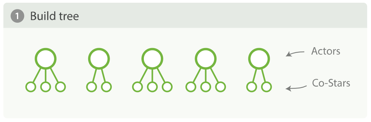
上述聚合分析,只是希望得到前10位演员和与他们联合出演者,但是为了得到最终的结果,我们创建了一个有 n * n 桶的树,然后对其排序,取 top10。如果我们有 2 亿doc,想要得到前 100 位演员以及与他们合作最多的 20 位演员,可以推测,聚合出来的分组数非常大。上述这种遍历方式就是深度优先。
4.8.2. 广度优先
Elasticsearch 允许我们改变聚合的集合模式,深度优先的方式对于大多数聚合都能正常工作,但对于上述情形就不太适用。为了应对这些特殊的应用场景,我们应该使用另一种集合策略叫做广度优先。这种策略的工作方式有些不同,它先执行第一层聚合,然后先做修剪,再执行下一层聚合。在我们的示例中,actors 聚合会首先执行,在这个时候,我们的树只有一层,但我们已经知道了前 10 位的演员,这就没有必要保留其他的演员信息,因为它们无论如何都不会出现在前十位中。 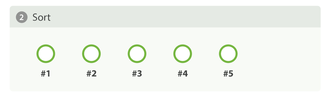
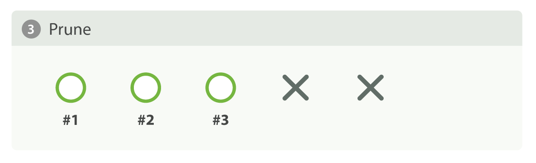
要使用广度优先,只需简单的通过参数 collect_mode 开启:
{
  "aggs" : {
    "actors" : {
      "terms" : {
         "field" : "actors",
         "size" : 10,
         "collect_mode" : "breadth_first"
      },
      "aggs" : {
        "costars" : {
          "terms" : {
            "field" : "actors",
            "size" :  5
          }
        }
      }
    }
  }
}
广度优先仅仅适用于每个组的聚合数量远小于当前总组数的情况,因为广度优先会在内存中缓存裁剪后的每个组的所有数据,如果裁剪后的每个组下的数据量非常大,广度优先就不是一个好的选择,这也是为什么深度优先作为默认策略的原因。

若有收获,就点个赞吧
0 人点赞
