It’s a beautiful Monday morning, and you just stepped into work after a relaxing weekend. After all, you just finished pdCalc on Friday, and now you are ready to ship. Before you can sit down and have your morning cup of coffee, your project manager steps into your office and says, “We’re not done. The client requested some new features.”
这是一个美丽的周一早晨,在经历了一个轻松的周末之后,你刚刚踏入工作岗位。毕竟,你在周五刚刚完成了pdCalc,现在你已经准备好发货了。在你坐下来喝早间咖啡之前,你的项目经理走进你的办公室,说:”我们还没有完成。客户要求一些新的功能”。
The above scenario is all too common in software development. While new features probably won’t be requested on the go live date, new features will almost inevitably be requested well after you have completed large parts of both your design and your implementation. Therefore, one should develop as defensively as practical to anticipate extensibility. I say as defensively as practical rather than as defensively as possible because overly abstract code can be as much of a detriment to development as overly concrete code. Often, it is easier to simply rewrite inflexible code if the need arises than it is to maintain highly flexible code for no reason. In practice, we seek to strike a balance for code to be both simple and maintainable yet somewhat extensible.
上述情况在软件开发中太常见了。虽然新的功能可能不会在上线之日被要求,但新的功能几乎不可避免地会在你完成设计和实现的大部分之后被要求。因此,我们应该尽可能地防御性地开发,以预见到可扩展性。我说尽可能地防御,而不是尽可能地防御,因为过于抽象的代码和过于具体的代码一样,都会对开发造成损害。通常情况下,如果有需要,简单地重写不灵活的代码要比无缘无故地维护高度灵活的代码更容易。在实践中,我们寻求一种平衡,使代码既简单、可维护又有一定的可扩展性。
In this chapter, we’ll explore modifying our code to implement features beyond the design of the original requirements. The discussion of the new features introduced in this chapter ranges from full design and implementation to design only to suggestions merely for self-exploration. Let’s begin with two extensions that we’ll take from requirements all the way through implementation.
在这一章中,我们将探讨修改我们的代码以实现超出原始需求设计的功能。本章介绍的新功能的讨论范围从完整的设计和实现,到仅有的设计,再到仅仅是自我探索的建议。让我们从两个扩展开始,我们将从需求一直到实现。
8.1 Fully Designed New Features 全面设计的新功能
In this section, we’ll examine two new features: batch operation of the calculator and execution of stored procedures. Let’s begin with batch operation.
在本节中,我们将研究两个新功能:计算器的批量操作和存储过程的执行。让我们从批量操作开始。
8.1.1 Batch Operation 批量操作
For those few unfamiliar with the term, batch operation of any program is simply the execution of the program, from beginning to end, without interaction from the user once the program is launched. Most desktop programs do not run in batch mode. However, batch operation is still very important in many branches of programming, such as scientific computing. Perhaps of greater interest, for those of you employed by large corporations, your payroll is probably run by a program operating in batch mode.
对于那些不熟悉这个术语的人来说,任何程序的批处理操作都是在程序启动后,在没有用户互动的情况下,从头到尾执行程序。大多数桌面程序不在批处理模式下运行。然而,批处理操作在编程的许多分支中仍然非常重要,如科学计算。也许更有意思的是,对于那些受雇于大公司的人来说,你们的工资单可能是由一个以批处理模式运行的程序来完成的。
Let’s be honest. Batch operation for pdCalc, other than maybe for testing, is not a very useful extension. I’ve included it mainly because it demonstrates how trivially a well-designed CLI can be extended to add a batch mode.
让我们说实话吧。pdCalc的批处理操作,除了可能用于测试之外,并不是一个非常有用的扩展。我把它包括在内,主要是因为它展示了一个设计良好的CLI是如何通过简单的扩展来增加批处理模式的。
Recall from Chapter 5 that pdCalc’s CLI has the following public interface:
回顾第五章,pdCalc的CLI有如下公共接口。
#endif // MODELINGGEOMETRY_Hclass Cli : public UserInterface {class CliImpl;public:Cli(istream& in, ostream& out);~Cli();void execute(bool suppressStartupMessage = false, bool echo = false);};
To use the CLI, the class is constructed with cin and cout as the arguments, and execute() is called with empty arguments:
为了使用CLI,该类是以cin和cout为参数构建的,而execute()是以空参数调用的。
Cli cli { cin, cout };// setup other parts of the calculatorcli.execute();
How do we modify the Cli class to enable batch operation? Amazingly, we do not need to modify the class’s code at all! By design, the CLI is essentially a parser that simply takes space-separated character input from an input stream, processes the data through the calculator, and generates character output to an output stream. Because we had the forethought not to hard code these input and output streams as cin and cout, we can convert the CLI to a batch processor by making the input and output streams to be file streams as follows:
我们如何修改Cli类以实现批量操作?令人惊讶的是,我们根本不需要修改该类的代码! 根据设计,CLI本质上是一个解析器,它只需从输入流中获取空格分隔的字符输入,通过计算器处理数据,并生成字符输出到输出流。因为我们有先见之明,没有把这些输入和输出流硬编码为cin和cout,所以我们可以通过使输入和输出流成为文件流,将CLI转换为一个批处理程序,如下所示。
ifstream fin { inputFile };ofstream fout { outputFile };Cli cli { fin, fout };// setup other parts of the calculatorcli.execute(true, true);
where inputFile and outputFile are file names that could be acquired through command line arguments to pdCalc. Recall that the arguments to the execute() function simply suppress the startup banner and echo commands to the output.
其中inputFile和outputFile是文件名,可以通过命令行参数获得pdCalc。回顾一下,execute()函数的参数只是抑制了启动时的横幅,并将命令回传到输出。
Yes, that really is it (but see main.cpp for a few implementation tricks). Our CLI was built originally so that it could be converted to a batch processor simply by changing its constructor arguments. You could, of course, argue that I, as the author, intentionally designed the Cli class this way because I knew the calculator would be extended in this manner. The reality is, however, that I simply construct all of my CLI interfaces with stream inputs rather than hard coded inputs because this design makes the CLI more flexible with nearly no additional cognitive burden.
是的,真的就是这样(但请看main.cpp中的一些实现技巧)。我们的 CLI 最初是这样构建的:只需改变其构造参数,就可以将其转换为一个批处理程序。当然,你可以说我,作为作者,故意这样设计Cli类,因为我知道计算器会以这种方式被扩展。然而现实是,我只是用流输入而不是硬编码输入来构建我所有的CLI接口,因为这种设计使CLI更加灵活,几乎没有额外的认知负担。
Before leaving this section, I’ll quickly note that the reality is that pdCalc’s CLI, with an assist from the operating system, already had a batch mode. By redirecting input and output at the command line, we can achieve the same results:
在离开这一节之前,我想快速地指出,现实是,pdCalc的CLI在操作系统的协助下,已经有了批处理模式。通过在命令行重定向输入和输出,我们可以达到同样的效果。
my_prompt> cat inputFile | pdCalc --cli > outputFile
For Windows, simply replace the Linux cat command with the Windows type command.
对于Windows,只需将Linux的cat命令替换为Windows的type命令。
8.1.2 Stored Procedures 存储程序
Adding a batch mode to pdCalc was, admittedly, a somewhat contrived example. The added functionality was not terribly useful, and the code changes were trivial. In this section, we’ll examine a more interesting feature extension: stored procedures.
诚然,给pdCalc增加一个批处理模式是一个有点矫揉造作的例子。增加的功能并不十分有用,而且代码的修改也是微不足道的。在本节中,我们将研究一个更有趣的功能扩展:存储过程。
What is a stored procedure? In pdCalc, a stored procedure is a stored, repeatable sequence of operations that operate on the current stack. Stored procedures provide a technique to expand the calculator’s functionality by creating user-defined functions from existing calculator primitives. You can think of executing a stored procedure as being analogous to running a very simple program for the calculator. The easiest way to understand the concept is to consider an example.
什么是存储过程?在pdCalc中,存储过程是一个存储的、可重复的操作序列,对当前堆栈进行操作。存储过程提供了一种技术,通过从现有的计算器基元创建用户定义的功能来扩展计算器的功能。你可以把执行一个存储过程看作是类似于为计算器运行一个非常简单的程序。理解这一概念的最简单方法是考虑一个例子。
Suppose you need to frequently calculate the hypotenuse of a triangle. For the right triangle depicted in Figure 8-1, we can compute the length of the hypotenuse, c, using the Pythagorean formula:
假设你需要经常计算一个三角形的斜边。对于图8-1中描述的直角三角形,我们可以用勾股定理公式计算斜边的长度c。
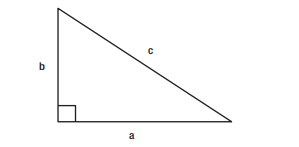
Figure 8-1. A right triangle
Suppose we had a triangle with sides a = 4, b = 3, and these values were entered onto pdCalc’s stack. In the CLI, you would see the following:
假设我们有一个边长为a=4,b=3的三角形,这些值被输入到pdCalc的栈中。在CLI中,你会看到下面的内容:
Top 2 elements of stack (size = 2):
堆栈的前2个元素(大小=2):
2: 3
1: 4
In order to compute c for this triangle, we would implement the following sequence of instructions: dup swap dup + 2 root. After pressing enter, the final result would be
为了计算这个三角形的c,我们将执行以下指令序列:dup swap dup + 2 root。按回车键后,最后的结果是
Top element of stack (size = 1):
堆栈的顶部元素(大小=1):
1: 5
If the commands were entered one at a time, we would see the intermediate resultant stack every time we pressed enter. Had we entered all of the commands on a single line and then pressed enter, pdCalc would display each intermediate stack before showing the final result. Note, of course, that this command sequence is not unique. The same result could have been achieved using, for example, the command sequence 2 pow swap 2 pow + 2 root.
如果命令是一个一个输入的,我们每次按回车键都会看到中间的结果堆。如果我们在一行中输入所有的命令,然后按回车键,pdCalc会在显示最终结果之前显示每个中间堆栈。当然,请注意,这个命令序列不是唯一的。例如,同样的结果也可以用2 pow交换2 pow+2 root的命令序列来实现。
If you are anything like me, if you had to compute hypotenuses with pdCalc repeatedly, you would probably want to automate the operation after the first manual computation. That is precisely what stored procedures allow. Not only does automation save time, but it is also less error-prone since stored procedures that encapsulate many consecutive commands can be written, tested, and subsequently reused. Provided the operation can be assembled from pdCalc primitives (including plugin functions), stored procedures enable extending the calculator’s functionality to compute simple formulas without needing to write any C++ code. Now we just need to design and implement this new feature.
如果你和我一样,如果你不得不用pdCalc重复计算下限,你可能会希望在第一次手动计算后实现自动化操作。这正是存储过程所允许的。自动化不仅可以节省时间,而且也不容易出错,因为封装了许多连续命令的存储过程可以被编写、测试,并随后被重复使用。只要操作可以由pdCalc基元(包括插件函数)组装而成,存储过程就可以扩展计算器的功能,计算简单的公式而不需要编写任何C++代码。现在我们只需要设计和实现这个新功能。
8.1.2.1 The User Interface
pdCalc has both a GUI and a CLI, so adding any user-facing feature will require some modification to both user interface components. For stored procedures, the modifications to the user interfaces are remarkably minor. First, a stored procedure is simply a text file containing an ordered sequence of pdCalc instructions. Therefore, a user can create a stored procedure using any plain text editor. Thus, unless you want to provide a stored procedure text editor with syntax highlighting, the user interface for stored procedures reduces to enabling their execution from the CLI and the GUI.
Let’s first address incorporating stored procedures in the CLI. As previously stated, stored procedures are simply text files in the file system. Recall that the CLI works by tokenizing space-separated input and then passing each token individually to the command dispatcher by raising an event. Therefore, a trivial method for accessing a stored procedure is simply to pass the name of the stored procedure file to the CLI. This file name will then be tokenized like any other command or number and passed to the command dispatcher for processing. To ensure that the file name is interpreted by the command dispatcher as a stored procedure rather than a command, we simply prepend the symbol proc: to the file name and change the command dispatcher’s parser. For example, for a stored procedure named hypotenuse.psp, we would issue the command proc:hypotenuse.psp to the CLI. I adopted the file extension psp as a shorthand for pdCalc stored procedure. Naturally, the file itself is an ordinary ASCII text file containing a sequence of commands for calculating the hypotenuse of a right triangle, and you can use the .txt extension if you prefer.
Recall that the GUI is designed to pass commands to the command dispatcher identically to the CLI. Therefore, to use a stored procedure, we add a button that opens a dialog to navigate the file system to find stored procedures. Once a stored procedure is selected, we prepend proc: to the file name and raise a CommandEntered event. Obviously, you can make your stored procedure selection dialog as fancy as you would like. I opted for a simplistic design that permits typing the name of the file into an editable combo box. For ease of use, the combo box is prepopulated with any files in the current directory with a .psp extension.
8.1.2.2 Changes to the Command Dispatcher
Listing 8-1 is an abbreviated listing of CommandDispatcher’s executeCommand() function including the logic necessary for parsing stored procedures. The omitted portions of the code appear in Section 4.5.2.
Listing 8-1. CommandDispatcher’s executeCommand() Function
void CommandDispatcher::CommandDispatcherImpl::executeCommand(const string& command){// handle numbers, undo, redo, help in nested if// ...else if (command.size() > 6 && command.substr(0, 5) == "proc:"){auto filename = command.substr(5, command.size() - 5);handleCommand(MakeCommandPtr<StoredProcedure>(ui_, filename));}// else statement to handle Commands from CommandRepository// ...return;}
From the code above, we see that the implementation simply peels off the proc: from the string command argument to create the stored procedure filename, creates a new StoredProcedure Command subclass, and executes this class. For now, we’ll assume that making the StoredProcedure class a subclass of the Command class is the optimal design. I’ll discuss why this strategy is preferred and examine its implementation in the following sections. However, before we get there, let’s discuss this new overload of the MakeCommandPtr() function.
In Section 7.2.1, we first saw a version of MakeCommandPtr given by the following implementation:
using CommandPtr = std::unique_ptr<Command, decltype(&CommandDeleter)>;inline auto MakeCommandPtr(Command* p){return CommandPtr { p, &CommandDeleter };}
The above function is a helper function used to create CommandPtrs from raw Command pointers. This form of the function is used to create a CommandPtr from the cloning of an existing Command (e.g., as in CommandRepository::allocateCommand()):
auto p = MakeCommandPtr(command->clone());
Semantically, however, in CommandDispatcherImpl::executeCommand(), we see a completely different usage, which is to construct an instance of a class derived from Command. Certainly, we can meet this use case with the existing MakeCommandPtr prototype. For example, we could create a StoredProcedure as follows:
auto c = MakeCommandPtr(new StoredProcedure { ui, filename });
However, whenever possible, it’s best not to pollute high-level code with naked news. We therefore seek to implement an overloaded helper function that can perform this construction for us. Its implementation is given by the following:
template <typename T, typename... Args>auto MakeCommandPtr(Args&&... args){return CommandPtr {new T { std::forward<Args>(args)... },&CommandDeleter};}
Prior to C++11, no simple and efficient technique existed for constructing generic types with variable numbers of constructor arguments, as is necessary to create any one of the possible classes derived from the Command class, each having different constructor arguments. Modern C++, however, provides an elegant solution to this problem using variadic templates and perfect forwarding. This construct is the subject of the sidebar below.
MODERN C++ DESIGN NOTE: VARIADIC TEMPLATES AND PERFECT FORWARDING
Variadic templates and perfect forwarding each solve different problems in C++. Variadic templates enable type-safe generic function calls with unknown numbers of typed arguments. Perfect forwarding enables correct type forwarding of arguments to underlying functions inside of template functions. The mechanics of each of these techniques can be studied in your favorite C++11 reference text (e.g., [23]). This sidebar shows a type-safe, generic design technique for constructing concrete objects that require different numbers of constructor arguments. This technique is enabled by the combination of variadic templates and perfect forwarding. Due to a lack of naming creativity, I named this pattern the generic perfect forwarding constructor (GPFC). Let’s begin by presenting the underlying problem that GPFC solves.
Let’s consider every author’s favorite overly simplified object-oriented programming example, the shapes hierarchy:
class Shape {public:virtual double area() const = 0;};class Circle : public Shape {public:Circle(double r): r_ { r }{}double area() const override { return 3.14159 * r_ * r_; }private:double r_;};class Rectangle : public Shape {public:Rectangle(double l, double w): l_ { l }, w_ { w }{}double area() const override { return l_ * w_; }private:double l_, w_;};
In C++, substitutability, implemented as virtual dispatch, solves the problem of needing to call a derived type’s specific implementation via a base class pointer using an interface guaranteed by the base class. In the shapes example, substitutability implies the ability to compute the area as follows:
double area(const Shape& s){return s.area();}
for any class derived from Shape. The exact interface for the virtual function is fully prescribed, including the number and type of any function arguments (even in the vacuous case as in the area() function in this example). The problem, however, is that object construction can never be “virtualized” in this manner, and even if it could, it wouldn’t work since the information necessary to construct an object (its arguments) is very frequently different from one derived class to the next.
Enter the generic perfect forwarding constructor pattern. In this pattern, we use variadic templates to provide a type-safe interface that can take any number of constructor arguments with different types. The first template argument is always the type we want to construct. Then, perfect forwarding is used to guarantee the arguments are passed to the constructor with the correct types. Precisely why perfect forwarding is necessary in this situation derives from how types are deduced in templates and is beyond the scope of this discussion (see [19] for details). For our shapes example, applying the GPFC pattern results in the following implementation:
template <typename T, typename... Args>auto MakeShape(Args&&... args){return make_unique<T>(forward<Args>(args)...);}
The following code illustrates how the MakeShape() function can be used to create different types with different numbers of constructor arguments:
auto c = MakeShape<Circle>(4.0);auto r = MakeShape<Rectangle>(3.0, 5.0);
Note that the GPFC pattern also works for creating classes not related to each other in an inheritance hierarchy. The GPFC pattern, in fact, is used by the make_unique() function in the standard library for making unique_ptrs in an efficient, generic manner without requiring a naked new. While they are, strictly speaking, distinct, I like to think of the GPFC pattern as the generic analogue of the factory method.
8.1.2.3 Designing the StoredProcedure Class
We now return to the thorny problem of designing the StoredProcedure class. The first question we ask is do we need a class at all. We already have a design for parsing individual commands, executing them, and placing them on an undo/redo stack. Maybe the correct answer is to treat a stored procedure in a manner similar to the treatment of batch input. That is, during an interactive session (either GUI or CLI), handle stored procedures by reading the stored procedure file, parsing it, and executing the commands in batch (as we would a long line with multiple commands in the CLI) without introducing a new StoredProcedure class.
The aforementioned design can be dismissed almost immediately after considering the following very simple example. Suppose you implemented a stored procedure for computing the area of a triangle. The stored procedure’s input would be the base and height of the triangle on the stack. triangleArea.psp is given by the following:
0.5
If we did not have a StoredProcedure class, then each of the commands in triangleArea.psp would be executed and entered, in order, on the undo/redo stack. For the values 4 and 5 on the I/O stack, forward execution of the stored procedure would yield the correct result of 10 and an undo stack, as depicted in Figure 8-2. Based on this undo stack, if the user tried to undo, rather than undoing the triangle area stored procedure, the user would undo only the top operation on the stack, the final multiply. The I/O stack would read
4
5
0.5
(and the undo stack would have a * between the 5 and 0.5) instead of
4
5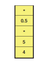
Figure 8-2. The undo stack without a StoredProcedure class
To fully undo a stored procedure, the user needs to press undo n times, where n is equal to the number of commands in the stored procedure. The same deficiency is present for the redo operation. In my opinion, the expected behavior for undoing a stored procedure should be to undo the entire procedure and leave the I/O stack in its state prior to executing the stored procedure. Hence, the design for handling stored procedures not employing a StoredProcedure class fails to implement undo and redo properly and must therefore be discarded.
8.1.2.4 The Composite Pattern
Essentially, in order to solve the undo/redo problem with stored procedures, we need a special command that encapsulates multiple commands but behaves as a single command. Fortunately, the composite pattern solves this dilemma. According to Gamma et al [6], the composite pattern “lets clients treat individual objects and compositions of objects uniformly.” Typically, the composite pattern refers to treed data structures. I prefer a looser definition where the pattern may be applied to any data structure admitting uniform treatment of composite objects.
Figure 8-3 illustrates the composite pattern in its general form. The Component class is an abstract class that requires some action to be performed. This action can be performed individually by a Leaf node or by a collection of Components known as a Composite. Clients interact with objects in the component hierarchy polymorphically through the Component interface. Both Leaf nodes and Composite nodes handle doSomething() requests indistinguishably from the client’s point of view. Usually, Composites implement doSomething() by simply calling the doSomething() command for Components (either Leafs or nested Composites) it holds.
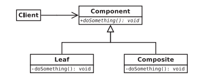
Figure 8-3. General form of the composite pattern
In our particular concrete case, the Command class takes the role of the Component, concrete commands such as Add or Sine take the role of Leaf nodes, and the StoredProcedure class is the composite. The doSomething() command is replaced by the executeImpl() and undoImpl() pair of pure virtual functions. I suspect combining the command and composite patterns in this fashion is rather common.
Previously, we learned that in order to properly implement the undo/redo strategy for stored procedures, a class design was necessary. Application of the composite pattern, as described above, motivates subclassing the StoredProcedure class from the Command class.
Let’s now design a StoredProcedure class and examine its implementation as a concrete application of the composite pattern.
8.1.2.5 A First Attempt
A common approach to implementing the composite pattern is via recursion. The Composite class holds a collection of Components, often either via a simple vector or perhaps something more complex such as nodes in a binary tree. The Composite’s doSomething() function simply iterates over this collection calling doSomething() for each Component in the collection. The Leaf nodes’ doSomething() functions actually do something and terminate the recursion. Although not required, the doSomething() function in the Component class is often pure virtual.
Let’s consider the above approach for implementing the composite pattern for StoredProcedures in pdCalc. We have already established that pdCalc’s Command class is the Component and that the concrete command classes, such as Add, are the Leaf classes. Therefore, we need only to consider the implementation of the StoredProcedure class itself. Note that since the current implementation of the Component and Leaf classes can be used as is, the composite pattern can be trivially applied to extend the functionality of an existing code base.
Consider the following skeletal design for the StoredProcedure class:
class StoredProcedure : public Command {private:void executeImpl() noexcept override;void undoImpl() noexcept override;vector<unique_ptr<CommandPtr>> components_;};
The executeImpl() command would be implemented as follows :
void StoredProcedure::executeImpl(){for (auto& i : components_)i->execute();return;}
undoImpl() would be implemented analogously but with a reverse iteration over the component_ collection.
Does the above design solve the undo/redo problem previously encountered when entering stored procedure commands directly onto the undo/redo stack without a StoredProcedure class? Consider the undo stack shown in Figure 8-4 for the triangleArea.psp example that we previously examined. The stored procedure, shown as SP in the figure, appears as a single object in the undo stack rather than as individual objects representing its constituent commands. Hence, when a user issues an undo command, the CommandManager will undo the stored procedure as a single command by calling the stored procedure’s undoImpl() function. This stored procedure’s undoImpl() function, in turn, undoes the individual commands via iteration over its container of Commands. This behavior is precisely what was desired, and this application of the composite pattern indeed solves the problem at hand. 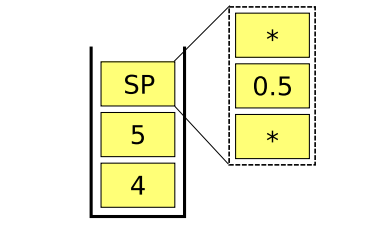
Figure 8-4. The undo stack using a StoredProcedure class
To complete the implementation of the StoredProcedure class, we need to parse the stored procedure file’s string commands (with error checking) and use them to populate the StoredProcedure’s components_ vector. This operation could be written in the StoredProcedure’s constructor, and the implementation would be both valid and complete. We would now have a StoredProcedure class that could transform string commands into Commands, store them in a container, and be able to execute and undo these stored Commands on demand. In other words, we would have essentially rewritten the command dispatcher! Instead, let’s consider an alternative design that implements the StoredProcedure class by reusing the CommandDispatcher class.
8.1.2.6 A Final Design for the StoredProcedure Class
The goal in this design is to reuse the CommandDispatcher class as-is. Relaxing this constraint and modifying the CommandDispatcher’s code can clean up the implementation slightly, but the essence of the design is the same either way. Consider the following modified skeletal design of the StoredProcedure class:
class StoredProcedure : public Command {private:void executeImpl() noexcept override;void undoImpl() noexcept override;std::unique_ptr<Tokenizer> tokenizer_;std::unique_ptr<CommandDispatcher> ce_;bool first_ = first;};
The present design is almost identical to our previous design except the components_ vector has been replaced by a CommandDispatcher, and the need for a tokenizer has been made explicit. Good thing we wrote our tokenizer to be reusable in Chapter 5!
We are now prepared to see the complete implementations of executeImpl() and undoImpl(). Note that while the below implementation does not use the canonical version of the pattern seen above, this implementation of the StoredProcedure class is still simply an application of the composite pattern. First, let’s examine executeImpl():
void StoredProcedure::executeImpl() noexcept{if (first_) {for (auto c : *tokenizer_) {ce_->commandEntered(c);}first_ = false;} else {for (unsigned int i = 0; i < tokenizer_->nTokens(); ++i)ce_->commandEntered("redo");}return;}
The first time that executeImpl() is called, the tokens must be extracted from the tokenizer and executed by the StoredProcedure’s own CommandDispatcher. Subsequent calls to executeImpl() merely request the StoredProcedure’s CommandDispatcher to redo the forward execution of each of the StoredProcedure’s commands. Remember, StoredProcedure’s executeImpl() function will itself be called by pdCalc’s CommandDispatcher; hence, our design calls for nested CommandDispatchers. Figure 8-5 shows this design for the triangle area stored procedure example, where CD represents the CommandDispatcher. 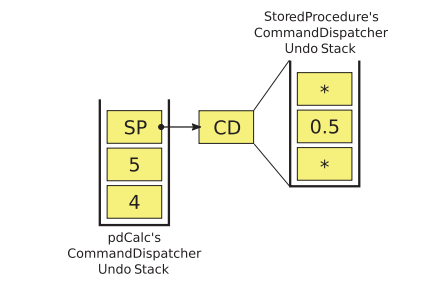
Figure 8-5. The undo stack using nested CommandDispatchers
The implementation of StoredProcedure’s undoImpl() is trivial:
void StoredProcedure::undoImpl() noexcept{for (unsigned int i = 0; i < tokenizer_->nTokens(); ++i)ce_->commandEntered("undo");return;}
Undo is implemented by requesting the underlying CommandDispatcher to undo the number of commands in the stored procedure.
Before concluding our discussion of the final StoredProcedure class, we should consider tokenization of the commands within the StoredProcedure class. The tokenization process for a StoredProcedure involves two steps. The stored procedure file must be opened and read, followed by the actual tokenization of the text stream. This process needs to be performed only once per StoredProcedure instantiation, at initialization. Therefore, the natural placement for tokenization is in the StoredProcedure’s constructor. However, placement of tokenization in the StoredProcedure’s constructor creates an inconsistency with pdCalc’s error handling procedure for commands. In particular, pdCalc assumes that commands can be constructed, but not necessarily executed, without failure. If a command cannot be executed, the expectation is that this error is handled by checking a command’s preconditions. Can tokenization fail? Certainly. For example, tokenization would fail if the stored procedure file could not be opened. Therefore, in order to maintain consistency in error handling, we implement tokenization in StoredProcedure’s checkPreconditionsImpl() function, which will be called when pdCalc’s CommandDispatcher first attempts to execute the stored procedure. Since tokenization needs to be performed once, we only perform the operation on the first execution of the checkPreconditionsImpl() function. The complete implementation can be found in the StoredProcedure.cpp file.
8.2 Designs Toward a More Useful Calculator
Up until now, all of the discussion about pdCalc has focused on the design and implementation of a completed code available for download from GitHub. The remainder of this chapter, however, marks a departure from this style. Henceforth, we will discuss only ideas for extensions and suggestions for how pdCalc might be modified to accommodate these new features. Not only is working code not provided, but working code was not created before writing these sections. Therefore, the designs I’m about to discuss have not been tested, and the adventurous reader choosing to complete these extensions may discover the ideas to be discussed are suboptimal, or, dare I say, wrong. Welcome to the wild west of designing features from a blank slate! Experimentation and iteration will be required.
8.2.1 Complex Numbers
The original design specification for the calculator called for double precision numbers, and we designed and implemented the calculator explicitly to handle only double precision numbers. However, requirements change. Suppose your colleague, an electrical engineer, drops by your office, falls in love with your calculator, but requires a calculator that handles complex (imaginary) numbers. That’s a reasonable request, so let’s look at how we might refactor our calculator to satisfy this new feature.
Adding complex numbers requires four main modifications to pdCalc: using a complex number representation internally instead of representing numbers as doubles, changing input and output (and, by extension, parsing) to accommodate complex numbers, modifying pdCalc’s stack to store complex numbers instead of doubles, and modifying commands to perform their calculations on complex numbers instead of real valued inputs. The first change, finding a C++ representation for complex numbers is trivial; we’ll use std::complex
8.2.1.1 Modifying Input and Output
Of all the required changes, modifying the I/O routines is actually the easiest. The first item to be addressed is how will complex numbers be interpreted and presented. For example, do we want a complex number, c, to be represented as c = re + im * i (maybe the imaginary number should be j since the feature request came from an electrical engineer). Perhaps we prefer using c = (re, im) or a variant that uses angle brackets or square brackets instead. There is no correct answer to this question. Although some choices might be easier to implement than others, since this choice is merely a convention, in practice, we would defer resolution to our customer. For our case study, we’ll simply adopt the convention c = (re, im).
I’ll only discuss modifying the command line version of the I/O. Once the infrastructure to handle complex numbers is in place for the CLI, adapting the GUI should be reasonably straightforward. The first problem that we encounter is the Tokenizer class. The original design for this class simply tokenized by splitting input on whitespace. However, for complex numbers, this scheme is insufficient. For example, complex numbers would be tokenized differently based on whether or not a space was inserted after the comma.
At some point, input becomes sufficiently complex that you’ll need to employ a language grammar and migrate the simple input routines to a “real” scanner and parser (possibly using libraries such as lex and yacc). Some might argue that by adding complex numbers, we have reached this level of complexity. However, I think that we can probably scrape by with our existing simple input tokenizer if we modify the tokenize() routine to scan for the ( token and create one “number” token for anything between and including the opening and closing parenthesis. Obviously, we would need to perform some basic error checking to ensure correct formatting. Another alternative would be to decompose the input stream based on regular expression matching. This is essentially how lex operates, and I would investigate using lex or a similar library before writing a sophisticated scanner from scratch.
The next input problem we encounter is parsing of numbers in CommandDispatcherImpl’s executeCommand() function. Currently, a string argument (the token) is passed to this function, and the string is parsed to determine if it is a number or a command. Upon inspection, we can see that executeCommand() will work for complex numbers if we modify isNum() to identify and return complex numbers instead of floating point numbers. Finally, the EnterNumber command will need to be updated to accept and store a complex
That takes care of modifying the input routines, but how do we modify the output routines? Recall that the Cli class is an (indirect) observer of the Stack’s stackChanged() event. Whenever the Stack raises this event, Cli’s stackChanged() function will be called to output the current stack to the command line. Let’s examine how Cli::stackChanged() is implemented. Essentially, the CLI calls back to the stack to fill a container with the top nElements using the following function call:
auto v = Stack::Instance().getElements(nElements);
An ostringstream, oss, is then created and filled first with some stack metadata and then with the stack elements using the following code:
size_t j { v.size() };for (auto i = v.rbegin(); i != v.rend(); ++i) {oss << j << ":\t" << *i << "\n";--j;}
Finally, the oss’s underlying string is posted to the CLI. Amazingly enough, once Stack’s getElements() function is modified to return a vector
8.2.1.2 Modifying the Stack
In Chapter 3, we originally designed the calculator’s stack to operate only on double precision variables. Clearly, this limitation means the Stack class must now be refactored in order to handle complex numbers. At the time, we questioned the logic of hard coding the target data type for the stack, and I recommended not designing a generic Stack class. My suggestion was, in general, to not design generic interfaces until the first reuse case is clearly established.
Designing good generic interfaces is generally harder than designing specific types, and, from my personal experience, I’ve found that serendipitous reuse of code infrequently comes to fruition. However, for our Stack class, the time to reuse this data structure for another data type has come, and it is prudent, at this point, to convert the Stack’s interface into a generic interface rather than merely refactor the class to be hard coded for complex numbers.
Making the Stack class generic is almost as easy as you might expect. The first step is to make the interface itself generic by replacing explicit uses of double with our generic type T. The interface becomes
template <typename T>class Stack : private Publisher {public:static Stack& Instance();void push(T, bool suppressChangeEvent = false);double pop(bool suppressChangeEvent = false);void swapTop();std::vector<T> getElements(size_t n) const;void getElements(size_t n, std::vector<T>&) const;using Publisher::attach;using Publisher::detach;};
With a generic interface, using the pimpl pattern is no longer necessary. Recall that use of the pimpl pattern enables us to hide the implementation of a class by referring to its implementation indirectly via a pointer to an implementation class defined only in a source file. However, in order to make the Stack generic, its implementation must also be generic (since it must store any type, T, rather than the single known type, double). This implies that StackImpl would also need to be templated. C++ rules insist that this StackImpl
In general, the required implementation changes are straightforward. Uses of double are replaced with T, and the implementation itself is moved to the header file. Uses of the Stack class within pdCalc obviously must be refactored to use the generic rather than the non-templated interface.
The last part of the interface that requires modification is the five global extern “C” helper functions added in Chapter 7 for exporting stack commands to plugins. Because these functions must have C linkage, we cannot make them templates nor can they return the C++ complex type in place of a double. The first problem is not quite as dire as it may appear at first glance. While our goal is to make the Stack class generic and reusable, the stack’s plugin interface does not need to be generic. For any particular version of pdCalc, either one that operates on real numbers or one that operates on complex numbers, only one particular instantiation of Stack
Replacing the complex
struct Complex {double re;double im;};
to complement the interface functions, replacing the current use of double with Complex. While this new Complex struct does duplicate the storage of the standard complex class, we cannot use the standard complex class in a pure C interface.
8.2.1.3 Modifying Commands
Modifying commands to work with complex numbers is really quite easy since the C++ library provides overloads for all of the mathematical operations required by our calculator. Minus the syntactic changes of replacing Stack with Stack
8.2.2 Variables
Earlier in this chapter, we implemented stored procedures as a method for storing a simple instruction sequence. While stored procedures work fine for trivial operations that only use each input once (e.g., the Pythagorean theorem), you’ll very quickly run into problems trying to implement more complicated formulas that use each input more than once (e.g., the quadratic formula). To overcome this difficulty, you’ll need to implement the ability to store arguments in named variables.
Implementing variables in pdCalc will require several modifications to existing components, including the addition of one prominent new component, a symbol table. For simplicity in the example code, I have reverted to using a real number representation for pdCalc. However, using complex numbers would add no additional design complexity. Let’s now explore some possible design ideas for implementing variables.
8.2.2.1 Input and New Commands
Obviously, using variables will require some means of providing symbolic names. Currently, our calculator only accepts numbers and commands as input. Inputting any string that cannot be found in the CommandRepository results in an error. Recall, however, that this error is generated in the CommandDispatcher, not in the tokenizer. Therefore, we need to modify the CommandDispatcher to not reject strings but instead to somehow place them on the stack. For now, we’ll assume that the stack can accept strings in addition to numbers. I’ll discuss the necessary modifications to the Stack class in the upcoming sections. Again, I’ll restrict our discussion to the command line interface. The only additional complication posed by the graphical user interface is providing a mechanism to input character strings in addition to numbers (perhaps a virtual keyboard to accompany the virtual numeric keypad).
Technically, we could allow any string to represent a variable. However, we are probably better served by restricting the allowable syntax to some subset of strings, possibly delimited by a symbol to differentiate variable names from commands. Because this choice is merely convention, you are free to choose whatever rules suit yours or your users’ tastes. Personally, I would probably choose something like variable names must begin with a letter and can contain any combination of letters, numbers, and possibly a few special symbols such as the underscore. To eliminate confusion between variable names and commands, I would enclose variables in either single or double quotation marks.
Now that we’ve established the syntax for variables, we’ll still need a mechanism for taking a number from the stack and storing it into a variable. The simplest method for accomplishing this task is to provide a new binary command, store, that removes a number and a string from the stack and creates a symbol table entry linking this variable name to this number. For example, consider the stack
4.5
2.9
“x”
Issuing the store command should result in an entry of x → 2.9 in the symbol table and a resultant stack of
4.5
Implicitly, variables should be converted to numbers for use during calculations but appear as names on the stack. We should also provide an explicit command, eval, to convert a symbolic name into a number. For example, given the stack
“x”
issuing the eval command should result in the stack
2.9
Such a command should have a fairly obvious implementation: replace the variable on the top of the stack with its value from the symbol table. Obviously, requesting the evaluation of a variable not in the symbol table should result in an error. Evaluating a number can either result in an error or, preferably, just return the number. You can probably think of any number of fancy commands for working with variables (e.g., list the symbol table). However, store and eval commands comprise the minimum necessary command set to use variables.
8.2.2.2 Number Representation and the Stack
Until now, our stack has only needed to represent a single, unique type, either a real or complex number. However, since variables and numbers can both be stored on the stack, we need the ability for the stack to store both types simultaneously. We dismiss immediately the notion of a stack that could handle two distinct types simultaneously because this would lead quickly to chaos. Instead, we seek a uniform representation capable of handling both number and variable types through a single interface. Naturally, we turn to a hierarchy.
Consider the design expressed in the class diagram in Figure 8-6. This hierarchy enables both Variables and Numbers to be used interchangeably as Values. This polymorphic design solves three problems that we’ve already encountered. First, Variables and Numbers can both be stored uniformly in a Stack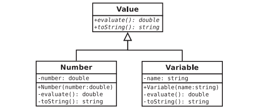
Figure 8-6. A hierarchy capable of representing both numbers and variables uniformly
8.2.2.3 The Symbol Table
At its core, a symbol table is merely a data structure that allows symbolic lookup by pairing a key to a value (an associative array). In this case, the name of the variable serves as the key and the numeric value serves as the value. The C++ standard library provides this service directly through either a map or an unordered_map, depending on the desired underlying data structure. However, as in Chapter 3, I highly recommend against directly using a standard library container as an external facing interface within a program. Instead, one should employee the adapter pattern to encapsulate the library container behind an interface defined by the application itself. This pattern adds no restrictions to the users of a class, but it does permit the designer to restrict, expand, or later modify the component’s interface independently of the interface of the underlying library container.
Therefore, the recommended design for a symbol table is to create a SymbolTable class to wrap an unordered_map
8.2.2.4 A Trivial Extension: Numeric Constants
Once we’ve established the mechanics for storing user-defined variables, we can make a trivial extension to provide user-defined constants. Constants are simply variables that cannot be altered once set. Constants could be hard coded in pdCalc, added at program launch through reading a constants file, or added dynamically during calculator execution.
Obviously, in order to store a constant, we will need to add a new command; let’s call it cstore. cstore works identically to store except that the command informs the symbol table that the variable being stored cannot be changed. We have two obvious options for implementation. First, inside the SymbolTable class, we add a second map that indicates whether a given name represents a variable or a constant. The advantage of this approach is that adding an additional map will require minimal implementation changes to the existing code. The disadvantage is that this approach requires two independent lookups for each call to the symbol table. The better approach is to modify the original map to store the value type as an Entry instead of a double, where an Entry is defined as
struct Entry {double val;bool isConst;};
Of course, to avoid hard coding the double type, we could, of course, template both SymbolTable and Entry.
8.2.2.5 Functionality Enabled by Variables
Let’s examine what variables enable us to do. Consider the quadratic equation  with roots given by
Where we formerly could not write a stored procedure for computing both roots, we can now write the stored procedure
“c” store “b” store “a” store “b” 2 pow 4 “a” “c” - sqrt “root” store “b” - “root” + 2 a / “b” - “root” 2 a /
which will take three entries from the stack representing the coefficients a, b, c and return two entries representing the roots of the quadratic equation. Now our calculator is getting somewhere!
8.3 Some Interesting Extensions for Self-Exploration
This chapter concludes with a section listing a few interesting extensions to pdCalc that you might consider trying on your own. In contrast to the previous section, I offer no design ideas to get you started. I have provided merely a brief description of each challenge.
8.3.1 High DPI Scaling
Monitors with extremely high pixel resolutions are becoming increasingly the norm. Consider how you would modify the GUI for pdCalc to properly handle scaling for such displays. Is this feature operating system independent or do we have another use for the PlatformFactory from Chapter 7? Since version 5.6, Qt helps you out with this task via an interface for high DPI scaling
8.3.2 Dynamic Skinning
In Chapter 6, a class was introduced to manage the look-and-feel of the GUI. However, the provided implementation only centralized the look-and-feel. It did not permit user customization.
Users often want to customize the look-and-feel of their applications. Applications that permit such changes are considered “skinable,” and each different look-and-feel is a called a skin. Consider an interface and the appropriate implementation changes necessary to the LookAndFeel class to enable skinning of pdCalc. Some possible options include a dialog for customizing individual widgets or a mechanism to choose skins from skin configuration files. Having a centralized class to handle the look-and-feel for the application should make this change straightforward. Don’t forget to add a signal to LookAndFeel so the other GUI elements will know when they need to repaint themselves with a new appearance!
8.3.3 Flow Control
With variables, we greatly enhanced the flexibility of stored procedures. For computing most formulas, this framework should prove sufficient. However, what if we wanted to implement a recursive formula such as computing the factorial of a number? While we have the ability to perform such complex computations via plugins, it would be nice to extend this functionality to users of the calculator who are not also experienced C++ programmers. To accomplish this task, we would need to devise a syntax for flow control. The simplest design would at least be able to handle looping and conditional operations. Adding flow control to pdCalc would be a fairly significant enhancement in terms of both added capability and implementation effort. It might be time to move to a real scanner and parser!
8.3.4 An Alternative GUI Layout
The pdCalc GUI currently has a vertical orientation inspired by the HP48S calculator. However, modern screen resolutions tend to be wider than they are tall, making the vertical orientation suboptimal. Hard coding a horizontal orientation is no more challenging than the original vertical orientation. Consider instead how to redesign pdCalc to be able to switch between orientations at runtime. Maybe vertical orientation is simply a different skin option?
8.3.5 A Graphing Calculator
The HP48 series of calculators were not merely scientific calculators, they were graphing calculators. Although it might not be practical to implement a graphing calculator for a computer when sophisticated standalone graphing programs exist, the exercise might prove to be a lot of fun. Starting with version 5.7, Qt now includes a graphing module to make this task significantly easier than it would have been previously. Given this graphing widget set, the biggest challenge might simply be devising a method for graphical input. If you’re in the mood for a silly throwback to the 1970s, consider implementing an ASCII graphing calculator for the CLI!
8.3.6 A Plugin Management System
Currently, plugins are loaded during pdCalc’s startup, and which plugins to load are determined by reading shared library names from a text file. Plugins, once loaded, cannot be unloaded. Consider implementing a dynamic plugin management system so that plugins can be selected, loaded, and unloaded at runtime. You could even extend the plugin interface to enable dynamic querying of plugin descriptions. I think the real gotcha here will be in figuring out how to handle the unloading of a plugin that has one of its commands currently on the undo/redo stack.
8.3.7 A Mobile Device Interface
In my original machinations for creating this book, I envisioned a chapter describing how to extend pdCalc to an iOS or Android tablet. The Qt library can once again help you with this task. The reason I did not include such a chapter in this book is that I do not have any practical experience with tablet programming. I felt it would be disingenuous to try to teach others how to design a tablet interface from my first-ever foray into that design space. Well, it might have been an excellent example of a bad design! Nonetheless, extending pdCalc to a tablet or smartphone interface is a worthy challenge, and the last one I leave you with.

若有收获,就点个赞吧
0 人点赞
