Complete and hand in this completed worksheet (including its outputs and any supporting code outside of the worksheet) with your assignment submission. For more details see the assignments page on the course website.
In this exercise you will:
- implement a fully-vectorized loss function for the SVM
- implement the fully-vectorized expression for its analytic gradient
- check your implementation using numerical gradient
- use a validation set to tune the learning rate and regularization strength
- optimize the loss function with SGD
- visualize the final learned weights
# Run some setup code for this notebook.import randomimport numpy as npfrom cs231n.data_utils import load_CIFAR10import matplotlib.pyplot as plt# This is a bit of magic to make matplotlib figures appear inline in the# notebook rather than in a new window.%matplotlib inlineplt.rcParams['figure.figsize'] = (10.0, 8.0) # set default size of plotsplt.rcParams['image.interpolation'] = 'nearest'plt.rcParams['image.cmap'] = 'gray'# Some more magic so that the notebook will reload external python modules;# see http://stackoverflow.com/questions/1907993/autoreload-of-modules-in-ipython%load_ext autoreload%autoreload 2
The autoreload extension is already loaded. To reload it, use:%reload_ext autoreload
CIFAR-10 Data Loading and Preprocessing
# Load the raw CIFAR-10 data.cifar10_dir = 'cs231n/datasets/cifar-10-batches-py'# Cleaning up variables to prevent loading data multiple times (which may cause memory issue)try:del X_train, y_traindel X_test, y_testprint('Clear previously loaded data.')except:passX_train, y_train, X_test, y_test = load_CIFAR10(cifar10_dir)# As a sanity check, we print out the size of the training and test data.print('Training data shape: ', X_train.shape)print('Training labels shape: ', y_train.shape)print('Test data shape: ', X_test.shape)print('Test labels shape: ', y_test.shape)
Clear previously loaded data.Training data shape: (50000, 32, 32, 3)Training labels shape: (50000,)Test data shape: (10000, 32, 32, 3)Test labels shape: (10000,)
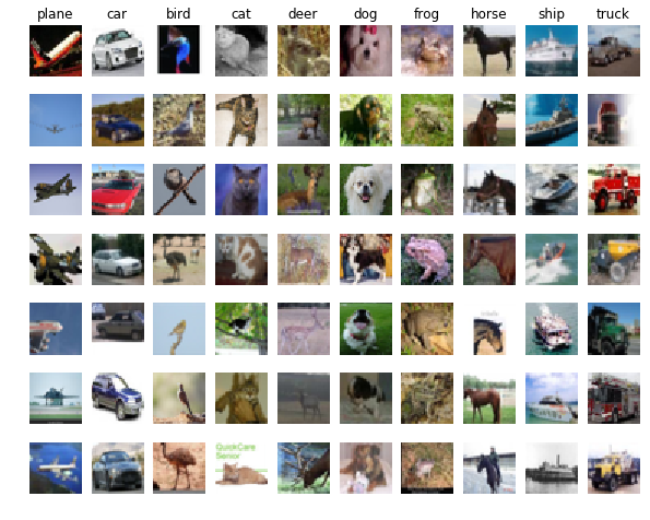
# Visualize some examples from the dataset.# We show a few examples of training images from each class.classes = ['plane', 'car', 'bird', 'cat', 'deer', 'dog', 'frog', 'horse', 'ship', 'truck']num_classes = len(classes)samples_per_class = 7for y, cls in enumerate(classes):idxs = np.flatnonzero(y_train == y)idxs = np.random.choice(idxs, samples_per_class, replace=False)for i, idx in enumerate(idxs):plt_idx = i * num_classes + y + 1plt.subplot(samples_per_class, num_classes, plt_idx)plt.imshow(X_train[idx].astype('uint8'))plt.axis('off')if i == 0:plt.title(cls)plt.show()
# Split the data into train, val, and test sets. In addition we will# create a small development set as a subset of the training data;# we can use this for development so our code runs faster.num_training = 49000num_validation = 1000num_test = 1000num_dev = 500# Our validation set will be num_validation points from the original# training set.mask = range(num_training, num_training + num_validation)X_val = X_train[mask]y_val = y_train[mask]# Our training set will be the first num_train points from the original# training set.mask = range(num_training)X_train = X_train[mask]y_train = y_train[mask]# We will also make a development set, which is a small subset of# the training set.mask = np.random.choice(num_training, num_dev, replace=False)X_dev = X_train[mask]y_dev = y_train[mask]# We use the first num_test points of the original test set as our# test set.mask = range(num_test)X_test = X_test[mask]y_test = y_test[mask]print('Train data shape: ', X_train.shape)print('Train labels shape: ', y_train.shape)print('Validation data shape: ', X_val.shape)print('Validation labels shape: ', y_val.shape)print('Test data shape: ', X_test.shape)print('Test labels shape: ', y_test.shape)
Train data shape: (49000, 32, 32, 3)Train labels shape: (49000,)Validation data shape: (1000, 32, 32, 3)Validation labels shape: (1000,)Test data shape: (1000, 32, 32, 3)Test labels shape: (1000,)
# Preprocessing: reshape the image data into rowsX_train = np.reshape(X_train, (X_train.shape[0], -1))X_val = np.reshape(X_val, (X_val.shape[0], -1))X_test = np.reshape(X_test, (X_test.shape[0], -1))X_dev = np.reshape(X_dev, (X_dev.shape[0], -1))# As a sanity check, print out the shapes of the dataprint('Training data shape: ', X_train.shape)print('Validation data shape: ', X_val.shape)print('Test data shape: ', X_test.shape)print('dev data shape: ', X_dev.shape)
Training data shape: (49000, 3072)Validation data shape: (1000, 3072)Test data shape: (1000, 3072)dev data shape: (500, 3072)
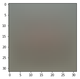
# Preprocessing: subtract the mean image# first: compute the image mean based on the training datamean_image = np.mean(X_train, axis=0)print(mean_image[:10]) # print a few of the elementsplt.figure(figsize=(4,4))plt.imshow(mean_image.reshape((32,32,3)).astype('uint8')) # visualize the mean imageplt.show()# second: subtract the mean image from train and test dataX_train -= mean_imageX_val -= mean_imageX_test -= mean_imageX_dev -= mean_image# third: append the bias dimension of ones (i.e. bias trick) so that our SVM# only has to worry about optimizing a single weight matrix W.X_train = np.hstack([X_train, np.ones((X_train.shape[0], 1))])X_val = np.hstack([X_val, np.ones((X_val.shape[0], 1))])X_test = np.hstack([X_test, np.ones((X_test.shape[0], 1))])X_dev = np.hstack([X_dev, np.ones((X_dev.shape[0], 1))])print(X_train.shape, X_val.shape, X_test.shape, X_dev.shape)
[130.64189796 135.98173469 132.47391837 130.05569388 135.34804082131.75402041 130.96055102 136.14328571 132.47636735 131.48467347]
(49000, 3073) (1000, 3073) (1000, 3073) (500, 3073)
SVM Classifier
Your code for this section will all be written inside cs231n/classifiers/linear_svm.py.
As you can see, we have prefilled the function compute_loss_naive which uses for loops to evaluate the multiclass SVM loss function.
# Evaluate the naive implementation of the loss we provided for you:from cs231n.classifiers.linear_svm import svm_loss_naiveimport time# generate a random SVM weight matrix of small numbersW = np.random.randn(3073, 10) * 0.0001loss, grad = svm_loss_naive(W, X_dev, y_dev, 0.000005)print('loss: %f' % (loss, ))print('shape of grad: ',grad.shape)
loss: 8.702263shape of grad: (3073, 10)
The grad returned from the function above is right now all zero. Derive and implement the gradient for the SVM cost function and implement it inline inside the function svm_loss_naive. You will find it helpful to interleave your new code inside the existing function.
To check that you have correctly implemented the gradient correctly, you can numerically estimate the gradient of the loss function and compare the numeric estimate to the gradient that you computed. We have provided code that does this for you:
# Once you've implemented the gradient, recompute it with the code below# and gradient check it with the function we provided for you# Compute the loss and its gradient at W.loss, grad = svm_loss_naive(W, X_dev, y_dev, 0.0)# Numerically compute the gradient along several randomly chosen dimensions, and# compare them with your analytically computed gradient. The numbers should match# almost exactly along all dimensions.from cs231n.gradient_check import grad_check_sparsef = lambda w: svm_loss_naive(w, X_dev, y_dev, 0.0)[0]grad_numerical = grad_check_sparse(f, W, grad)# do the gradient check once again with regularization turned on# you didn't forget the regularization gradient did you?loss, grad = svm_loss_naive(W, X_dev, y_dev, 5e1)f = lambda w: svm_loss_naive(w, X_dev, y_dev, 5e1)[0]grad_numerical = grad_check_sparse(f, W, grad)
numerical: -2.097039 analytic: -2.097039, relative error: 1.632850e-12numerical: -13.150595 analytic: -13.150595, relative error: 8.383147e-12numerical: 35.293383 analytic: 35.293383, relative error: 1.306768e-11numerical: 11.074474 analytic: 11.074474, relative error: 2.002911e-11numerical: 9.746951 analytic: 9.746951, relative error: 1.532373e-11numerical: -0.897797 analytic: -0.897797, relative error: 1.196728e-11numerical: -7.943663 analytic: -7.943663, relative error: 2.130405e-11numerical: -16.034647 analytic: -16.034647, relative error: 1.573243e-11numerical: 8.443374 analytic: 8.443374, relative error: 1.431563e-11numerical: -3.365248 analytic: -3.365248, relative error: 1.020220e-10numerical: -18.147710 analytic: -18.147710, relative error: 6.067783e-13numerical: -11.426479 analytic: -11.426479, relative error: 6.281970e-12numerical: -3.141528 analytic: -3.141528, relative error: 1.164299e-10numerical: 0.282185 analytic: 0.282185, relative error: 7.727437e-10numerical: -10.892570 analytic: -10.892570, relative error: 7.020010e-12numerical: -3.616890 analytic: -3.616890, relative error: 2.809321e-11numerical: -30.501798 analytic: -30.501798, relative error: 3.546797e-12numerical: -9.108684 analytic: -9.108684, relative error: 3.362022e-11numerical: 8.114566 analytic: 8.114566, relative error: 1.355445e-11numerical: 12.924950 analytic: 12.924950, relative error: 2.482065e-11
Inline Question 1
It is possible that once in a while a dimension in the gradcheck will not match exactly. What could such a discrepancy be caused by? Is it a reason for concern? What is a simple example in one dimension where a gradient check could fail? How would change the margin affect of the frequency of this happening? Hint: the SVM loss function is not strictly speaking differentiable
# Next implement the function svm_loss_vectorized; for now only compute the loss;# we will implement the gradient in a moment.tic = time.time()loss_naive, grad_naive = svm_loss_naive(W, X_dev, y_dev, 0.000005)toc = time.time()print('Naive loss: %e computed in %fs' % (loss_naive, toc - tic))from cs231n.classifiers.linear_svm import svm_loss_vectorizedtic = time.time()loss_vectorized, _ = svm_loss_vectorized(W, X_dev, y_dev, 0.000005)toc = time.time()print('Vectorized loss: %e computed in %fs' % (loss_vectorized, toc - tic))# The losses should match but your vectorized implementation should be much faster.print('difference: %f' % (loss_naive - loss_vectorized))
Naive loss: 8.702263e+00 computed in 0.078789sVectorized loss: 8.702263e+00 computed in 0.007735sdifference: -0.000000
# Complete the implementation of svm_loss_vectorized, and compute the gradient# of the loss function in a vectorized way.# The naive implementation and the vectorized implementation should match, but# the vectorized version should still be much faster.tic = time.time()_, grad_naive = svm_loss_naive(W, X_dev, y_dev, 0.000005)toc = time.time()print('Naive loss and gradient: computed in %fs' % (toc - tic))tic = time.time()_, grad_vectorized = svm_loss_vectorized(W, X_dev, y_dev, 0.000005)toc = time.time()print('Vectorized loss and gradient: computed in %fs' % (toc - tic))# The loss is a single number, so it is easy to compare the values computed# by the two implementations. The gradient on the other hand is a matrix, so# we use the Frobenius norm to compare them.difference = np.linalg.norm(grad_naive - grad_vectorized, ord='fro')print('difference: %f' % difference)
Naive loss and gradient: computed in 0.088396sVectorized loss and gradient: computed in 0.004990sdifference: 0.000000
Stochastic Gradient Descent
We now have vectorized and efficient expressions for the loss, the gradient and our gradient matches the numerical gradient. We are therefore ready to do SGD to minimize the loss.
# In the file linear_classifier.py, implement SGD in the function# LinearClassifier.train() and then run it with the code below.from cs231n.classifiers import LinearSVMsvm = LinearSVM()tic = time.time()loss_hist = svm.train(X_train, y_train, learning_rate=1e-7, reg=2.5e4,num_iters=1500, verbose=True)toc = time.time()print('That took %fs' % (toc - tic))
iteration 0 / 1500: loss 780.845025iteration 100 / 1500: loss 284.218950iteration 200 / 1500: loss 107.290724iteration 300 / 1500: loss 42.352389iteration 400 / 1500: loss 18.537910iteration 500 / 1500: loss 10.759981iteration 600 / 1500: loss 6.869571iteration 700 / 1500: loss 6.355614iteration 800 / 1500: loss 5.903678iteration 900 / 1500: loss 5.378417iteration 1000 / 1500: loss 5.844359iteration 1100 / 1500: loss 5.279668iteration 1200 / 1500: loss 5.036227iteration 1300 / 1500: loss 5.161794iteration 1400 / 1500: loss 4.938430That took 16.796489s
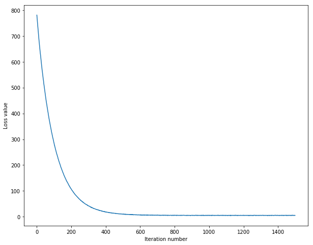
# A useful debugging strategy is to plot the loss as a function of# iteration number:plt.plot(loss_hist)plt.xlabel('Iteration number')plt.ylabel('Loss value')plt.show()
# Write the LinearSVM.predict function and evaluate the performance on both the# training and validation sety_train_pred = svm.predict(X_train)print('training accuracy: %f' % (np.mean(y_train == y_train_pred), ))y_val_pred = svm.predict(X_val)print('validation accuracy: %f' % (np.mean(y_val == y_val_pred), ))
training accuracy: 0.367388validation accuracy: 0.370000
# Use the validation set to tune hyperparameters (regularization strength and# learning rate). You should experiment with different ranges for the learning# rates and regularization strengths; if you are careful you should be able to# get a classification accuracy of about 0.39 on the validation set.# Note: you may see runtime/overflow warnings during hyper-parameter search.# This may be caused by extreme values, and is not a bug.from cs231n.classifiers import LinearSVMlearning_rates = np.linspace(1e-6,1e-8,5)regularization_strengths = np.linspace(4.5e4,5.5e4,5)# results is dictionary mapping tuples of the form# (learning_rate, regularization_strength) to tuples of the form# (training_accuracy, validation_accuracy). The accuracy is simply the fraction# of data points that are correctly classified.results = {}best_val = -1 # The highest validation accuracy that we have seen so far.# The LinearSVM object that achieved the highest validation rate.best_svm = None################################################################################# TODO: ## Write code that chooses the best hyperparameters by tuning on the validation ## set. For each combination of hyperparameters, train a linear SVM on the ## training set, compute its accuracy on the training and validation sets, and ## store these numbers in the results dictionary. In addition, store the best ## validation accuracy in best_val and the LinearSVM object that achieves this ## accuracy in best_svm. ## ## Hint: You should use a small value for num_iters as you develop your ## validation code so that the SVMs don't take much time to train; once you are ## confident that your validation code works, you should rerun the validation ## code with a larger value for num_iters. ################################################################################## *****START OF YOUR CODE (DO NOT DELETE/MODIFY THIS LINE)*****svm = LinearSVM()acc_temp = 0for lr in learning_rates:for reg in regularization_strengths:svm.train(X_train, y_train, learning_rate=lr, reg=reg,num_iters=150, verbose=True)train_acc = np.mean(y_train == svm.predict(X_train))val_acc = np.mean(y_val == svm.predict(X_val))results[(lr, reg)] = (train_acc, val_acc)if val_acc > acc_temp:best_val = val_accacc_temp = best_valbest_svm = svm# *****END OF YOUR CODE (DO NOT DELETE/MODIFY THIS LINE)*****# Print out results.for lr, reg in sorted(results):train_accuracy, val_accuracy = results[(lr, reg)]print('lr %e reg %e train accuracy: %.2f val accuracy: %.2f' % (lr, reg, train_accuracy, val_accuracy))print('best validation accuracy achieved during cross-validation: %f' % best_val)
iteration 0 / 150: loss 1396.757584iteration 100 / 150: loss 7.978646iteration 0 / 150: loss 7.074112iteration 100 / 150: loss 6.814321iteration 0 / 150: loss 6.906133iteration 100 / 150: loss 6.113737iteration 0 / 150: loss 6.380821iteration 100 / 150: loss 6.100835iteration 0 / 150: loss 6.743149iteration 100 / 150: loss 7.828594iteration 0 / 150: loss 7.270202iteration 100 / 150: loss 6.695549iteration 0 / 150: loss 5.911166iteration 100 / 150: loss 6.497495iteration 0 / 150: loss 6.323286iteration 100 / 150: loss 6.402935iteration 0 / 150: loss 6.360113iteration 100 / 150: loss 6.215709iteration 0 / 150: loss 6.329384iteration 100 / 150: loss 6.792598iteration 0 / 150: loss 7.810835iteration 100 / 150: loss 6.215014iteration 0 / 150: loss 6.047842iteration 100 / 150: loss 6.189011iteration 0 / 150: loss 5.712657iteration 100 / 150: loss 6.202888iteration 0 / 150: loss 6.219806iteration 100 / 150: loss 6.846721iteration 0 / 150: loss 5.953943iteration 100 / 150: loss 5.950440iteration 0 / 150: loss 5.930696iteration 100 / 150: loss 5.878044iteration 0 / 150: loss 5.672647iteration 100 / 150: loss 5.687492iteration 0 / 150: loss 5.630673iteration 100 / 150: loss 6.361494iteration 0 / 150: loss 5.624344iteration 100 / 150: loss 5.781926iteration 0 / 150: loss 5.934599iteration 100 / 150: loss 5.907119iteration 0 / 150: loss 6.388585iteration 100 / 150: loss 6.015466iteration 0 / 150: loss 6.002802iteration 100 / 150: loss 5.679754iteration 0 / 150: loss 5.205385iteration 100 / 150: loss 5.423794iteration 0 / 150: loss 5.784023iteration 100 / 150: loss 5.535814iteration 0 / 150: loss 5.612699iteration 100 / 150: loss 6.147560lr 1.000000e-08 reg 4.500000e+04 train accuracy: 0.36 val accuracy: 0.37lr 1.000000e-08 reg 4.750000e+04 train accuracy: 0.36 val accuracy: 0.38lr 1.000000e-08 reg 5.000000e+04 train accuracy: 0.36 val accuracy: 0.37lr 1.000000e-08 reg 5.250000e+04 train accuracy: 0.36 val accuracy: 0.37lr 1.000000e-08 reg 5.500000e+04 train accuracy: 0.36 val accuracy: 0.37lr 2.575000e-07 reg 4.500000e+04 train accuracy: 0.35 val accuracy: 0.34lr 2.575000e-07 reg 4.750000e+04 train accuracy: 0.35 val accuracy: 0.37lr 2.575000e-07 reg 5.000000e+04 train accuracy: 0.34 val accuracy: 0.36lr 2.575000e-07 reg 5.250000e+04 train accuracy: 0.34 val accuracy: 0.35lr 2.575000e-07 reg 5.500000e+04 train accuracy: 0.34 val accuracy: 0.37lr 5.050000e-07 reg 4.500000e+04 train accuracy: 0.32 val accuracy: 0.33lr 5.050000e-07 reg 4.750000e+04 train accuracy: 0.33 val accuracy: 0.32lr 5.050000e-07 reg 5.000000e+04 train accuracy: 0.32 val accuracy: 0.34lr 5.050000e-07 reg 5.250000e+04 train accuracy: 0.32 val accuracy: 0.31lr 5.050000e-07 reg 5.500000e+04 train accuracy: 0.31 val accuracy: 0.33lr 7.525000e-07 reg 4.500000e+04 train accuracy: 0.29 val accuracy: 0.31lr 7.525000e-07 reg 4.750000e+04 train accuracy: 0.31 val accuracy: 0.34lr 7.525000e-07 reg 5.000000e+04 train accuracy: 0.27 val accuracy: 0.28lr 7.525000e-07 reg 5.250000e+04 train accuracy: 0.29 val accuracy: 0.31lr 7.525000e-07 reg 5.500000e+04 train accuracy: 0.27 val accuracy: 0.28lr 1.000000e-06 reg 4.500000e+04 train accuracy: 0.28 val accuracy: 0.29lr 1.000000e-06 reg 4.750000e+04 train accuracy: 0.27 val accuracy: 0.28lr 1.000000e-06 reg 5.000000e+04 train accuracy: 0.26 val accuracy: 0.25lr 1.000000e-06 reg 5.250000e+04 train accuracy: 0.29 val accuracy: 0.28lr 1.000000e-06 reg 5.500000e+04 train accuracy: 0.26 val accuracy: 0.27best validation accuracy achieved during cross-validation: 0.377000
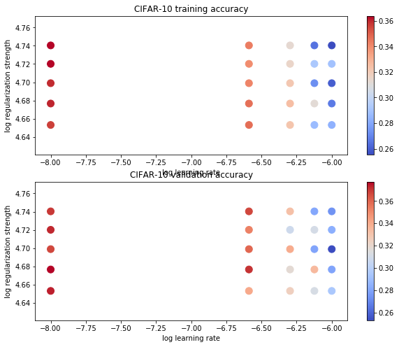
# Visualize the cross-validation resultsimport mathx_scatter = [math.log10(x[0]) for x in results]y_scatter = [math.log10(x[1]) for x in results]# plot training accuracymarker_size = 100colors = [results[x][0] for x in results]plt.subplot(2, 1, 1)plt.scatter(x_scatter, y_scatter, marker_size, c=colors, cmap=plt.cm.coolwarm)plt.colorbar()plt.xlabel('log learning rate')plt.ylabel('log regularization strength')plt.title('CIFAR-10 training accuracy')# plot validation accuracycolors = [results[x][1] for x in results] # default size of markers is 20plt.subplot(2, 1, 2)plt.scatter(x_scatter, y_scatter, marker_size, c=colors, cmap=plt.cm.coolwarm)plt.colorbar()plt.xlabel('log learning rate')plt.ylabel('log regularization strength')plt.title('CIFAR-10 validation accuracy')plt.show()
# Evaluate the best svm on test sety_test_pred = best_svm.predict(X_test)test_accuracy = np.mean(y_test == y_test_pred)print('linear SVM on raw pixels final test set accuracy: %f' % test_accuracy)
linear SVM on raw pixels final test set accuracy: 0.361000
# Visualize the learned weights for each class.# Depending on your choice of learning rate and regularization strength, these may# or may not be nice to look at.w = best_svm.W[:-1,:] # strip out the biasw = w.reshape(32, 32, 3, 10)w_min, w_max = np.min(w), np.max(w)classes = ['plane', 'car', 'bird', 'cat', 'deer', 'dog', 'frog', 'horse', 'ship', 'truck']for i in range(10):plt.subplot(2, 5, i + 1)# Rescale the weights to be between 0 and 255wimg = 255.0 * (w[:, :, :, i].squeeze() - w_min) / (w_max - w_min)plt.imshow(wimg.astype('uint8'))plt.axis('off')plt.title(classes[i])
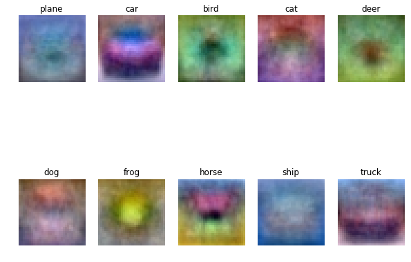
Inline question 2
Describe what your visualized SVM weights look like, and offer a brief explanation for why they look they way that they do.
!jupyter nbconvert --to markdown svm.ipynb
[NbConvertApp] Converting notebook svm.ipynb to markdown[NbConvertApp] Support files will be in svm_files\[NbConvertApp] Making directory svm_files[NbConvertApp] Making directory svm_files[NbConvertApp] Making directory svm_files[NbConvertApp] Making directory svm_files[NbConvertApp] Making directory svm_files[NbConvertApp] Writing 23693 bytes to svm.md

若有收获,就点个赞吧
0 人点赞
