英文名叫Numerical Analysis,简称NA。PTA上labs的测试点很变态,一道题debug一天,上CSDN看看往届学长学姐的思路会好一点。这门课本来不应该大一学的,但是我没能补选上C大程,只能拿这门课来凑学分了。折大早日被中科大救赎罢,请(无慈悲)
0. About This Course
**Course Code** 21190641**Instructor** 黄劲**Time** Spring & Summer, 2022**Course Goals** To give an introduction to classical approximation technique, to explain how, why, and when they can be expected to work, to provide a firm basis for future study of scientific computing.
1. Mathematical Preliminaries
1.1 Roundoff Error and Computer Arithmetic
数值分析中常用≈。如果出现=,那么应该是这样的形式:f(x) = 近似值 + 余项。
余项用 e 或 r 表示,e for error(误差) and r for remainder(余项)。近似值可用 f 表示。
描述余项(默认是大小未知的非负数)用的是它的上界。对于误差 e 和近似值 f ,有0 ≤ e ≤ ē和f* - ē ≤ f(x) ≤ f* + ē。下界总是0,因为如果下界是某正数,这正的一部分就是知道确切值的,就应该把这个大小已知的正数加到近似值里,再把下界调成0,只剩下大小不确定的部分。**Truncation Error** 截断误差,the error involved in using a truncated, or finite summation to approximate the sum of an infinite series.**Roundoff Error** 舍入误差,the error produced when performing real number calculations. It occurs because the arithmetic performed in a machine involves numbers with only a finite number of digits,电脑里面这么几个有限的二进制的位是很难表示出完备的实数运算的。**Normalized decimal floating-point form of a real number** (k-digit decimal machine number) is like ±0.d1d2…dk×10n where 1 ≤ d1 ≤ 9 and 0 ≤ di ≤ 9 (i = 2, 3, … , k).
If p is an approximation to p, the **absolute error**(绝对误差) is | p - p|, and the **relative error**(相对误差) is ![[已弃修]数值分析 - 图1](/uploads/projects/linguisty@zju_courses/26ea66d0719a28b81c64ea7f8e5b9dee.svg) , provided that p≠0.
, provided that p≠0.
The number p is said to approximate p to t `*significant digits (figures)`(有效数字) if t is the largest nonnegative integer for which ![[已弃修]数值分析 - 图2](/uploads/projects/linguisty@zju_courses/cc5d0da792dc9ac4d35cfc13ba0a0ab8.svg) < 5×10-t.
< 5×10-t.
📋舍入误差往往小于截断误差,原因如下: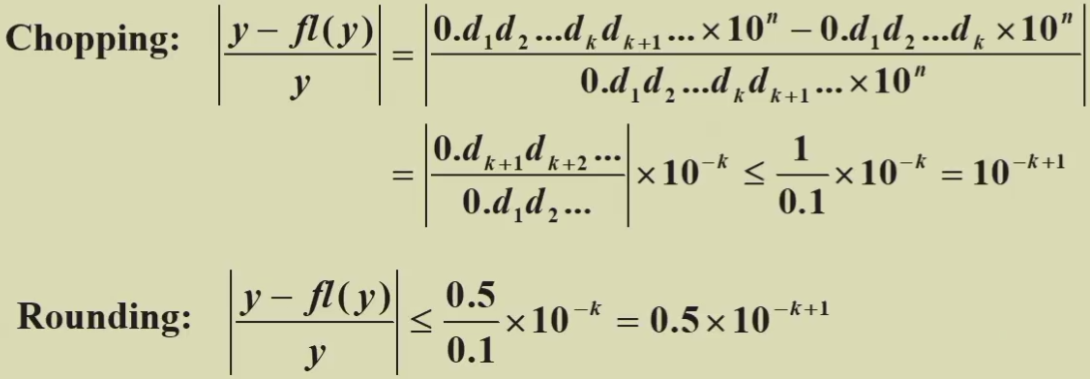
📋计算结果受误差影响的两种情况:
- 两个大小相近的数据作差会导致有效数字急剧减少,相对误差急剧增大。直接用 f(x) = f* + e 和相对误差的定义就能证明。
- Dividing by a number with small magnitude (or equivalently multiplying by a number with large magnitude) will cause an enlargement of the error.
💡除法是计算机中最危险的四则运算,计算机中出现巨大的数,往往是因为除法。
🌰e.g.
计算机中只有3位运算,那么每一步都只能用三位浮点数,每次出现超过3位的真实值都得近似,而不是中途精确计算,在最后出结果时取三位数就好了。
⚠️这里 truncation error 比 roundoff error 还小,这是很正常的。说 roundoff error 往往更小是因为误差上界更小,而在计算精度受限的情况下,我们并不知道误差确切的值是多少(要是知道的话,直接给近似值加上误差就得到精确值了,要近似值干什么呢?),误差确切的值可以视为一个概率函数。在概率上,roundoff error 小的可能性大,但是偶尔出现 truncation error 小的个例也是合理的。
1.2 Algorithms and Convergence
An algorithm that satisfies that small changes in the initial data produce correspondingly small changes in the final results is called **stable**; otherwise it is **unstable**. An algorithm is called **conditionally stable** if it is stable only for certain choices of initial data.
Suppose that E0 > 0 denotes an initial error and En represents the magnitude of an error after n subsequent operations. If En≈ C n E0 where C is a constant independent of n, then the growth of error is said to be **linear**. If E ≈ Cn E0, for some C > 1, then the growth of error is called **exponential**.
💡Linear growth of error is usually unavoidable, and when C and E0 are small the results are generally acceptable. Exponential growth of error should be avoided since the term Cn becomes large for even relatively small values of n. This leads to unacceptable inaccuracies, regardless of the size of E0. 而且很多情况下出现指数增长不是因为实际情形太复杂,而是因为代码写成了屎山(老师原话)。
💡每次计算,误差(当然也是指误差的范围/上界)都会积累,不论是线性增长还是指数增长。因此,往往计算次数少的算法误差更小(当然也是概率意义上的)。

2. Solutions of Equations in One Variable
2.1 The Bisection Method
📋The Intermediate Value Theorem(介值定理)
If f ∈ C[a, b] and K is any number between f(a) and f(b), then there exists a number p ∈ (a, b) for which f(p) = K.
📋Algorithm: Bisection(二分法)
就是数学分析中证明零点存在定理使用的算法。
Suppose that f ∈ C[a, b] and f(a) · fb)<0. The bisection method generates a sequence {pn} (n=0, 1, 2, ...) approximating a zero p of f with |pn - p| ≤ (b - a) / 2n
优点:
- 要求少,函数连续即可
- 一定能收敛
缺点:
- a、b初值不好取,需要对函数有足够多的先验信息才能用这个方法
- 收敛慢(数值分析中O(log n)的算法也认为是慢的)
-
2.2 Fixed-Point Iteration
f(x)=0 → g(x)=x
Root of f(x) → Fixed-Point of g(x)
📋Fixed-Point Theorem(不动点定理)
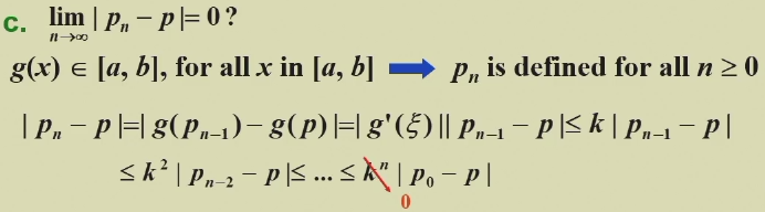
Let g ∈ C[a, b] be such that g(x) ∈ [a, b], for all x in [a, b]. Suppose, in addition, that g’ exists on (a, b) and that a constant 0<k<1 exists with |g’(x)| ≤ k for all x ∈ (a, b). Then, for any number p0 in [a, b], the sequence defined by pn=g(pn-1), n ≥ 1, converges to the unique fixed-point p in [a,b].
证明分三段:a. 不动点存在;b. 不动点唯一; c. 能收敛到不动点。
⚠️不直接写|g’(x)|<1是因为k是常数,可以防止出现g’(x)作为变量无限趋近1的情况。
📋Corollary: If g satisfies the hypotheses of the Fixed-Point Theorem, then bounds for the error involved in using pn to approximate p are given by (for all n ≥ 1):
📋Algorithm: Fixed-Point Iteration(不动点迭代)
2.3 Newton’s Method
Linearize a nonlinear function using Taylor’s expansion. 如图,选择初值p0,在p0处用直线拟合。如果初值选得好,直线和x轴的交点就会比初值更接近真实值p。

📋牛顿法收敛定理
Let f ∈ C2[a, b](二阶连续). If p ∈ [a, b] is such that f(p) = 0 and f ‘(p) ≠ 0,then there exists a δ > 0 such that Newton’s method generates a sequence {Pn}(n=1, 2, …) converging to p for any initial approximation p0 ∈ [p-δ, p+δ].![ZJWL13SFMJKYIU9UICDG9]Y.png](/uploads/projects/linguisty@zju_courses/253ee181859f9112ec66ad1fe731f5c4.png)

then { pn } (n = 0, 1, 2, …) converges to p of**order**(收敛阶) α, with**asymptotic error constant**(渐进误差常数)λ. The larger the value of α, the faster the convergence. If α =1, the sequence is linearly convergent.
- If α =2, the sequence is quadratically convergent.
📋Theorem
Let p be a fixed point of g(x). If there exists some constant α ≥ 2 such that g ∈ Cα [p – δ, p + δ], g’(p) = … = g(α – 1)(p) = 0, and g(α)(p) ≠ 0. Then the iterations with pn = g( pn – 1 ), n ≥ 1, is of order α.
Proof: 
2.5 Accelerating Convergence
For a given sequence { pn } (n = 1, 2, …), the **forward difference** Δpn is defined by Δpn = pn+1 – pn for n ≥ 0. Higher powers, Δkpn, are defined recursively by Δkpn = Δ(Δk-1pn ) for for k ≥ 2.
📋Aitken’s Δ2 Method
Construct a new sequence { p-hatn } based on { pn } like this, and it is supposed to converge to p faster than { pn }.
💡 p-hatn 的这个定义式背后的几何直观是这样的:
📋Theorem
Suppose that { pn } (n = 1, 2, …) is a sequence that converges linearly to the limit p and that for all sufficiently large values of n we have ( pn – p )( pn+1 – p ) > 0. Then the sequence { p-hatn } (n = 1, 2, …) converges to p faster than { pn } (n = 1, 2, …) in the sense that:

若有收获,就点个赞吧
0 人点赞
