10. Graph Theory
Graphs are mathematical abstracts of relations existing in some concrete things in the objective world.
10.1 Graphs and Graph Models
A **graph**  consists of
  , a nonempty set of
 **vertices** (or nodes), and  , a set of
 **edges**. Each edge has either one or two vertices associated with it, called its **endpoints**. An edge is said to connect its endpoints.
🌰 e.g.
 , where
  ,
, 
**Infinite graph**: A graph with an infinite vertex set or an infinite number of edges.**Finite graph**: A graph with a finite vertex set and a finite number of edges.
💡 We shall consider only finite graph in this course.
**Undirected graph**: A graph with undirected edges. Undirected graph can be classified into:
**Simple graph**: A graph in which each edge connects two different vertices and where no two edges connect the same pair of vertices.**Multigraph**: Graphs that may have multiple edges connecting the same vertices.**Pseudograph**: Graphs that may include loops, and possibly multiple edges connecting the same pair of vertices.

**Directed graph**: A graph with directed edges. A directed graph (or digraph)  consists of a nonempty set of vertices
  and a set of directed edges (or arcs)
  . Each directed edge is associated with an ordered pair of vertices. The directed edge associated with the ordered pair
  is said to start at
  and end at
  . Digraph can be classified into:
**Simple directed graph**: A directed graph has no loops and has no multiple directed edges.**Directed multigraph**: A directed graphs that may have multipledirected edges from a vertex to a second (possibly the same) vertex.
**Mixed graph**: A graph with both directed and directed edges.
⚙️ Problems in almost every conceivable discipline can be solved using **graph models**. For example:
- Ramsey Problem: Each pair of individuals consists of two friends or two enemies, show that there are either three mutual friends or three mutual enemies in the group of six people.
- Precedence Graph(前趋图)
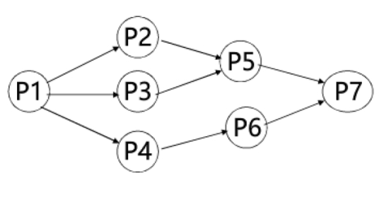
Precedence graphs represent the order of completing a series of tasks using directed graphs instead of Hasse graphs.
10.2 Graph Terminology and Special Types of Graphs
In Undirected Graphs  :
:
- Two vertices
 and
and  in an undirected graph
  are called
 **adjacent**(or**neighbors**) in , if
, if  is an edge of
  .
. - An edge
 connecting
  and
and  is called
 **incident**with vertices and
and  , or is said to
 **connect** and
and  .
. - The vertices
 and
and  are called
 **endpoints**of edge .
. - An edge connects a vertex to itself is called a
**loop**. - The
**neighborhood**of , denoted as
  , is the set of all neighbors of a vertex
  .
. - The
**degree**of a vertex in an undirected graph is the number of edges incident with it, except that a loop at a vertex contributes twice to the degree of that vertex. Notation: .
. - If
 ,
,  is called
 **isolated**. - If
 ,
,  is called
 **pendant**.
🌰 e.g.
Find the degree of all the vertices.
 ,
,  ,
,  ,
,  because
  is connected by a loop,
  ,
,  .
.
Total of degrees = 3 + 3 + 4 + 5 + 1 + 0 = 16.
📋 The Handshaking Theorem
Let  be an undirected graph with
  edges. Then
  .
.
🌰 e.g.
If a graph has 5 vertices, can each vertex have degree 3? 4?
Solution:
If each vertex have degree 3, then the sum is 3×5 = 15, which is an odd number, so it is not possible. If each vertex have degree 4, then it may be possible.
📋 Corollary: An undirected graph has an even number of vertices of odd degree.
In Directed Graphs  :
:
- Let
 be an edge in
  . Then
  is an
is an **initial vertex**and is**adjacent to** , and
, and  is a
is a **terminal vertex**and is**adjacent from** .
. - The
**in degree**of a vertex , denoted by
  , is the number of edges which terminate at
  . Similarly, the
 **out degree**of , denoted by
  , is the number of edges which initiate at
  .
. - The method of ignoring the directions in a digraph to find a path is called
**underlying undirected graph**.
📋 Let  be a graph with direct edges (not necessarily a digraph), then
  . If it is a directed graph, then
  .
.
📋 Some Special Simple Graphs
- Complete Graphs —
 : the simple graph with
  vertices and exactly one edge between every pair of distinct vertices.

- Cycles —
 :
:  , where
  ,
,  ,
,  .
.

- Wheels
 : Add one additional vertex to the cycle
  and add an edge from each vertex to the new vertex to produce
  .
.

⚠️ Note that  has
has  vertices.
- n-Cubes
 :
:  is the graph with
  vertices representing bit strings of length
  , where
  ,
,  .
.

📋 Construct  from
from 
- Making two copies of
 , prefacing the labels on the vertices with a 0 in one copy and with a 1 in the other copy.
 - Adding edges connecting two vertices that have labels differing only in the first bit.

A simple graph  is
is **bipartite**(偶图) if  can be partitioned into two disjoint subsets
  and
and  such that every edge connects a vertex in
  and a vertex in
  . The pair
  is called a
 **bipartition** of the vertex  of
of  . The
. The **complete bipartite graph** is the simple graph that has its vertex set partitioned into two subsets  and
and  with
with  and
and  vertices, respectively, and every vertex in
  is connected to every vertex in
  , denoted by
  , where
  and
and  .
.
📋 A simple graph is bipartite if and only if it is possible to assign one of two different colors to each vertex of the graph so that no two adjacent vertices are assigned the same color.
💡 如果简单图中存在一个由奇数个结点构成的回路,那么这个简单图不是偶图,因为必然会有两个相邻的结点被涂成相同的颜色。→ 奇数个齿轮啮合成一圈形成的结构不能转动,因为必然会有两个相邻的齿轮需要同向转动。
🌰

A simply graph is called **regular** if every vertex of this graph has the same degree. A regular graph is called **n-regular** if every vertex in this graph has degree  .
.
🌰 e.g. is a (n-1)-regular.
⚙️ Special types of graphs can be used to represent local area networks.
 ,
,  .
.  is a
is a **subgraph** of  if
if  and
and  . Subgraph
  is a
is a **proper subgraph** of  if
if  .
.  is a
is a **spanning subgraph** of  if
if  ,
,  .
.
🌰 e.g.
How many subgraphs with at least one vertex does  have?
have?
Solution:
Choose 1 to 4 vertices from the wheel each time, and decide whether there are vertices between each pair of the vertices.  .
.
⚠️ Note that here each vertex is considered to be different from others.
Let  be a simple graph. The subgraph
 **induced** by a subset  of the vertex set
  is the graph
  , where the edge set
  contains an edge in
  iff both endpoints of this edge are in
  .
.
📋 Graph Operation
- Removing edges of a graph:

- Adding edges to a graph:

**Edge contration**(边收缩): Remove an edge with endpoints
  and
and  , merge
  and
and  into a new single vertex
  , and for each edge with
  or
or  as an endpoint, replace the edge with one with
  as endpoint in place of
  and
and  and with the same second endpoint.


- Removing vertices from a graph:
 , where
  is the set of edges of
  not incident to
  .
. - The
**union**of two simple graphs and
and  is the simple graph with vertex set
  and edge set
  , denoted as
  .
.


10.3 Representing Graphs and Graph Isomorphism
10.3.1 Adjacency Lists
**Adjacency lists**(邻接表) are lists that specify the vertices that are adjacent to each vertex.
For simple graphs:
 |
Vertices | Adjacent Vertices |
|---|---|---|
| a | b, c, d | |
| b | a, d | |
| c | a, d | |
| d | a, b, c |
For digraphs:
 |
Initial Vertex | Terminal Vertices |
|---|---|---|
| a | c | |
| b | a | |
| c | ||
| d | a, b, c |
10.3.2 Adjacency Matrices
A simple graph  with
with  vertices
  can be represented by its
 **adjacency matrix**(邻接矩阵),  , where
  .
.
⚠️ Note that an adjacency matrix of a graph is based on the ordering chosen for the vertices.
 |
Adjacency Matrix | ||||
|---|---|---|---|---|---|
| a | b | c | d | ||
| a |  |
||||
| b | |||||
| c | |||||
| d |
To represent a multigraph or pseudograph using adjacency matrixes, just let the  -th entry of such a matrix equals the number of edges that are associated to
  .
.
⚠️ Note that a loop only contribute 1 to the corresponding entry.
 |
Adjacency Matrix | ||||
|---|---|---|---|---|---|
| a | b | c | d | ||
| a |  |
||||
| b | |||||
| c | |||||
| d |
📋 Adjacency matrices of undirected graphs are always symmetric.
For directed graph  with
with  , suppose that the vertices of
  are listed in arbitrary order as
  , the adjacency matrix
  , where
  .
.
 |
Adjacency Matrix | ||||
|---|---|---|---|---|---|
| a | b | c | d | ||
| a |  |
||||
| b | |||||
| c | |||||
| d |
📋 The sum of the entries in a row / column of the adjacency matrix for an undirected graph is the number of edges incident to the vertex  , which is the same as
  minus the number of loops at
  .
.
📋 The sum of the entries in a row of the adjacency matrix for an digraph is  . In a column it is
  .
.
💡 计算机中,考虑到占用空间大小,邻接表比较适合表示稀疏矩阵,而邻接矩阵比较适合表示稠密矩阵。
10.3.3 Incidence Matrices
 ,
,  ,
,  . Then the
 **incidence matrix** with respect to this ordering of  and
and  is
is  matrix
  , where
  .
.
 |
Incidence Matrix | ||||||
|---|---|---|---|---|---|---|---|
| 1 | 2 | 3 | 4 | 5 | 6 | ||
| a |  |
||||||
| b | |||||||
| c | |||||||
| d |
📋 Incidence matrices of undirected graphs contain two 1s per column for edges connecting two vertices, and one 1 per column for loops.
10.3.4 Isomorphism of Graphs
Two simple graphs  and
and  are
are **isomorphic**(同构) if there is a one-to-one correspondence function  (
( is called an
 **isomorphism**) from  to
to  such that for all
  and
and  in
in  ,
,  and
and  are adjacent in
  iff
iff  and
and  are adjacent in
  .
.
In other words, when two simple graphs are isomorphic, there is a one-to-one correspondence between vertices of the two graphs that preserves the adjacency relationship.
🌰 e.g.
Show that the following two graphs are isomorphic.
Proof:
- Try to find an isomorphism
 .
. - Show that
 preserves adjacency relation- The adjacency matrix of a graph
  is the same as the adjacency matrix of another graph
  , when rows and columns are labeled to correspond to the images under
  of the vertices in
  .
.
Here  and
and  are the same. So
  where
where  ,
,  ,
,  ,
,  ,
,  is a proper isomorphism.
It is usually difficult to find an isomorphism  since there are
  possible 1-1 correspondence between the two vertex sets with
  vertices.
However, there are some properties called **invariants**(不变量) in the graphs that may be used to show that they are not isomorphic. Graph invariants are properties preserved by isomorphism of graphs.
📋 Important Invariants in Isomorphic Graphs:
- the number of vertices
- the number of edges
- the degrees of corresponding vertices
- if one is bipartite, the other must be.
- if one is complete, the other must be.
- if one is a wheel, the other must be.
etc.
🌰 e.g.
Draw all nonisomorphic undirected simple graph with four vertices and three edges.
Solution:
By the handshaking theorem, the sum of the degrees over four vertices is 6. The maximal degree is 3, and the number of vertices with odd degrees must even. So there are 3 possible sequence of degrees:
(1) 1, 1, 2, 2; (2) 1, 1, 1, 3; (3) 0, 2, 2, 2.
10.4 Connectivity
10.4.1 Paths
A **path** of **length**  from
from  to
to  in an undirected graph is a sequence of
  edges
edges  for which there exists a sequence
  such that
  has endpoints
  . When the graph is simple, we denote this path by its vertex sequence
  . If the path begins and ends with the same vertex, we call it a
 **circuit**. The path or circuit is said to **pass through** the vertices  or
or **traverse** the edges  . If a path or a circuit does not contain the same edge more than once, we call it a
 **simple** path / circuit.
A **path** of length  from
from  to
to  in a directed graph is a sequence of edges
  such that
  is associated with
  , … ,
, … ,  is associated with
  , … ,
, … ,  is associated with
  . When there are no multiple edges in the directed graph, this path is denote by its vertex sequence
  . The definitions of circuit and simple path / circuit still holds in directed graphs.
An undirected graph is **connected** if there is a path between every pair of distinct vertices, and is **disconnected** if the graph is not connected. To **disconnect** a graph means to remove vertices or edges, or both, to produce a disconnected subgraph.
⚠️ is considered to be connected.
📋 There is a simple path between every pair of distinct vertices of a connected undirected graph.
Proof:
Since the graph is connected, there is a path between  and
and  . Throw out all redundant circuits to make the path simple.
The maximally connected subgraphs of  are called the
 **connected components** or simply “components”.
If removing a vertex and all edges incident with it results in more connected components than in the original graph, then it is called a **cut vertex** or an **articulation point**. If removing a edge creates more components, then it is called a **cut edge** or a **bridge**. Connected graphs without cut vertices are called **nonseparable graphs**.
Nonseparable graphs can be thought of as more connected than those with a cut vertex. We can measure graph connectivity based on the minimum number of vertices removed to disconnect a graph.
10.4.2 Connectivities in Undirected Graphs
Here  is a undirected graph.
A **vertex cut**, or **separating set**, is a subset  of the vertex set
  of
of  such that
  is disconnected or
  .
.
📋 Every connected graph except a complete graph has a vertex cut.
The **vertex connectivity**(点连通度) of  , denote as
  , is the minimum number of vertices in a vertex cut, or equivalently, the minimum number of vertices that can be removed from
  to either disconnect
  or produce a graph with a single vertex. The larger
  is, the more connected we consider
  to be. A graph is said to be
 **k-connected** (or k-vertex-connected ), if  .
.
is the 10th letter in Greek alphabet, called “kappa”.
📋 Properties of Vertex Connectivities
- If
 has
has  vertices, then
  .
. iff
iff  is disconnected or
  .
. if
if  is connected with cut vertices or
  .
. iff
iff  .
.
We can also measure graph connectivity based on the minimum number of edges removed to disconnect a graph.
A set of edges  is called an
 **edge cut** of  if the subgraph
  is disconnected.
The **edge connectivity**(边连通度) of  , denoted as
  , is the minimum number of edges in an edge cut of
  , or equivalently, the minimum number of edges removed from
  to disconnect
  .
.
📋 Properties of Edge Connectivities
- If G has n vertices, then
 .
. if
if  is disconnected or
  .
. iff
iff  .
.
📋 Whitney’s Inequality(惠特尼不等式)
When  is a noncomplete connected graph with at least three vertices,
  .
.
💡 去掉结点的时候会把连接到这个点的边一起去掉。去点的同时也在去边,所以去点对连通度的影响比单纯去边的影响大,所以点连通度比边连通度小。不需要会证,记得有这么个结论就行。
⚙️ Vertex and edge connectivity can be used to analysis the reliability of network. The vertex connectivity of the graph representing network equals the minimum number of routers that disconnect the network when they are out of service. The edge connectivity represents the minimum number of fiber optic links that can be down to disconnect the network.
10.4.3 Connectivities in Digraphs
Here  is a digraph.
 is said to be
 **strongly connected** if there is a path from  to
to  and from
  to
to  for all vertices
  and
and  . If the underlying undirected graph is connected, then we say it is
 **weakly connected**.
⚠️ By the definition, any strongly connected directed graph is also weakly connected.
For directed graph, the maximal strongly connected subgraphs are called the **strongly connected components** or just the **strong components**.
🌰 e.g.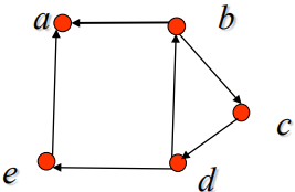
There are 3 strong components in this digraph:
 .
. .
.- The subgraph consisting of vertices
 ,
,  , and
, and  and edges
  ,
,  ,
,  .
.
💡 定义可达性矩阵: ,其中
,其中 为 1 表示存在一条从结点 i 到 j 的路径,为 0 表示不存在。那么
 就是原有向图的邻接矩阵的传递闭包。
10.4.4 Applications of Paths
📋 Two graphs are isomorphic only if they have simple circuits of the same length.
📋 Two graphs are isomorphic only if they contain paths that go through vertices so that the corresponding vertices in the two graphs have the same degree.
🌰 e.g.
Are these two graphs isomorphic?
Solution:
They are not, because the right graph contains circuits of length 3, while the left graph does not.
📋 The number of different paths of length  from
from  to
to  is equal to the
  th entry of
  (the standard power of
  , not the Boolean product), where
  is the adjacency matrix representing the graph consisting of vertices
  .
.
Proof:
The proof is based on MI. Let  .
.
Basic Step:  .
.
Inducive Case: Assuming that the  th entry of
  is the number of different paths of length
  from
from  to
to  . Then for
  , let
, let  , then
  , where
  is the number of paths of length
  passing the vertex
  .
.
🌰 e.g.
How many paths of length 2 are there from
 to
to  ?
?Solution:
 in
in  is 1.
is 1.The number of paths not exceeding 6 are there from
 to
to  ?
?Solution:
 in
in  is 2.
is 2.The number of circuits starting at vertex
 whose length is not exceeding 6?
10.5 Euler and Hamilton Paths
10.5.1 Euler Path
**Euler Path**: A simple path containing every edge of . 这里 simple 的意思是同一条边不能走多次,也就是说 Euler path 解决的是一笔画问题。
**Euler Circuit**: A simple circuit containing every edge of .
.**Euler Graph**: A graph contains an Euler circuit.
📋 Necessary and Sufficient Condition for Euler Circuits and Paths
A connected multigraph has an Euler circuit ↔ each of its vertices has even degree.
Proof:
(1) has an Euler circuit ⇒ Every vertex in
  has even degree
Consider the Euler circuit starting and ending at vertex :
:
 in
in  is 2.
is 2.
- First edge of the Euler circuit contributes one to the degree of
 .
. - Each time the circuit passes through a vertex it contributes two to the vertex’s degree
- The circuit terminates where it started, contributing one to
 .
.
(2) Every vertex in  has even degree ⇒ We can form a Euler circuit that begins at an arbitrary vertex
  of
of 
- Build a simple circuit
 .
. - An Euler circuit has been constructed if all the edges have been used. Otherwise:
- Construct a simple path in the subgraph
 obtained from
  . Let
. Let  be a vertex which is the common vertex of the circuit and
  . Beginning at
  , construct a simple path in
  .
. - Form a circuit in
 by splicing the circuit in
  with the original circuit in
  .
. - Continue this process until all edges have been used.
- (Explained in detail later)
📋 A connected multigraph has an Euler path but not an Euler circuit ↔ It has exactly two vertices of odd degree.
Proof:
(1) Suppose the multigraph has an Euler path from  to
to  .
.
- The first edge of the Euler path contributes one to the degree of
 .
. - The last edge in the Euler path contributes one to the degree of
 .
. - The path contributes two to the degree of a vertex whenever it passes through it.
(2) Suppose that a graph has exactly two vertices of odd degree, say  and
and  .
.
- Add an edge
 , then every vertex has even degree, so there is an Euler circuit.
 - The removal of the new edge produces an Euler path.
🌰 e.g.
Königsberg Seven Bridge Problem:
Is it possible to pass each of the 7 bridges(represented as edges in the graph) exactly once?
Solution:
The graph has four vertices of odd degree. Therefore, it does not have an Euler circuit. It does not have an Euler path either.
📋 An algorithm to find an Euler path or Euler circuit in a given graph
PROCEDURE Euler (G: connected and all vertices of even degree)circuit := a circuit in G beginning at an arbitraryily chosen vertex withedges successively added to form a path that return to this vertexH := G with the edges of this circuit removedWHILE H has edgesBEGINsubcircuit := a circuit in H beginning at a vertex in H that is also anendpoint of an edge of circuitH := H with edges of subcircuit and all isolated vertices removedcircuit := circuit with subcircuit inserted at the appropriate vertexEND {circuit is an Euler circuit}
To form an Euler path in a graph without an Euler circuit, we follow the procudure above as well, but start and end at the two vertices of odd degrees.
🌰 e.g.
Determine whether the following graph has an Euler path. Construct such a path if it exists.
| 1 | 2 | 3 |
|---|---|---|
 |
 |
 |
| ACEABCDEGJ | ACEABCDEGJ+EFGIJE =ACEFGIJEABCDEGJ |
ACEFGIJEABCDEGHIGJ+GHIG =ACEFGIJEABCDEGHIGJ |
Solution:
The graph has exactly 2 vertices of odd degree, and all of the other vertices have even degree. Therefore, this graph has an Euler path.
The concept of Euler cuicuit can be extended to digraphs.
📋 A directed multigraph having no isolated vertices has an Euler circuit if and only if:
- The graph is weakly connected.
- The in-degree and out-degree of each vertex are equal.
📋 A directed multigraph having no isolated vertices has an Euler path but not an Euler circuit if and only if:
- The graph is weakly connected.
- The in-degree and out-degree of each vertex are equal for all but two vertices, one that has in-degree 1 larger than its out-degree and the other that has out-degree 1 larger than its in-degree.
⚙️ Application of Euler Paths
- One-Stroke Problem

Draw a picture in a continuous motion without lifting the pencil so that no part of the picture is retraced. The problem is equivalent to deciding whether there is a Euler path and constructing the path if it exists.
Some route planning problems, where we need to avoid retracing a road, are equivalent to a one-stroke problem.
- The Chinese Postman Problem (CPP)
中国邮递员问题是邮递员在某一地区的信件投递路程的问题。邮递员每天从邮局出发,走遍该地区所有街道再返回邮局,那么他应如何安排送信的路线可以使所走的总路程最短?这个问题由中国学者管梅谷在1960年首先提出,并给出了解法——“奇偶点图上作业法”。用图论的语言描述,就是给定一个连通图 ,每边
,每边 有非负权,要求一条回路经过每条边至少一次,且满足总权最小。
10.5.2 Hamilton’s Paths
**Hamilton Path**: A path which visits every vertex in  exactly once.
**Hamilton Circuit**: A cycle which visits every vertex exactly once, except for the first vertex, which is also visited at the end of the cycle.**Hamilton Graph**: A connected graph  with a Hamilton circuit
The definitions apply both to undirected as well as directed graphs of all types.
The idea of Hamilton path rose from Hamilton’s puzzle, where we try passing every vertex of a graph without passing any vertex twice.")
Currently, there are no useful necessary and sufficient conditions for the existence of Hamilton circuit. A few sufficient conditions have been found.
📋 Dirac’s Theorem(迪拉克定理)
If  is a simple graph with
  vertices with
  such that the degree of every vertex in
  is at least
  , then
  has a Hamilton path.
📋 Ore’s Theorem(奥尔定理)
If  is a simple graph with
  vertices with
  such that
  for every pair of nonadjacent vertices
  and
and  in
in  , then
  has a Hamilton circuit.
💡 这两个定理的核心理念就是:有足够多的边的图中存在哈密顿道路/回路。
📋 Certain properties can be used to show that a graph has no Hamilton circuit:
- A graph with a vertex of degree one cannot have a Hamilton circuit.
- A graph with a cut vertex cannot have a Hamilton circuit.
- If a vertex in the graph has degree two, then both edges that are incident with this vertex must be part of any Hamilton circuit.
- When a Hamilton circuit is being constructed and this circuit has passed through a vertex, then all remaining edges incident with this vertex, other than the two used in the circuit , can be removed from consideration.
📋 Another Important Necessary Condition
If there is a Hamilton circuit in  , for any nonempty subset
  of set
  , the number of connected components in
  is less than or equal to
  . 可以这么记:有哈密顿回路说明这个图是连通的,每去掉一个结点就能产生一个新的连通分支已经是最极端的情况了。
🧷 Note:
Suppose that  is a H circuit of
  . For any nonempty subset
  of set
  , the number of connected components in
  is less than or equal to
  , and the number of connected components in
  is less than or equal to the number of connected components in
  . 可以这么记:
 中可能去掉了一些
 中有的边,所以连通性只能比
 差,连通分支数量一定不少于
 。
。
⚙️ Hamilton path or circuit can be used to solve many practical problems, including the famous TSP (Traveling Salesperson Problem), where the salesperson wants to reach every city exactly once.
🌰 e.g.
Seating Problem: There are seven people denoted by A, B, C, D, E, F, G. Suppose that the following facts are known.
- A — English (A can speak English.)
- B — English, Chinese
- C — English, Italian, Russian
- D — Japanese, Chinese
- E — German, Italia
- F — French, Japanese, Russian
G — French, German
How to arrange seat for the round desk such that the seven people can talk each other?
Solution:

- Construct a graph
 , where
  ,
, 
- If there is a H circuit, then we can arrange seat for the round desk such that the seven people can talk each other. The H circuit is
 .
.
🌰 e.g.
Seven examination must be arranged in a week. Each day has one examination. The examinations are in charged by the same teacher cannot be arranged in the adjacent two days. One teacher is in charge at most four examinations. Show that the arrangement is possible.
Proof:
- Construct graph, where
 : seven examination,
- If there is a Hamilton path, then the arrangement is possible. Since one teacher is in charge at most four examinations, then every vertex in the graph has at least three adjacent vertices. It follows that the sum of the degrees of a pair vertices is at least 6.
According to Ore’s theorem, there is a H circuit connecting 6 of the vertices. By removing an edge and connect an endpoint to the 7th vertex, we get a H path.
10.6 Shortest Path Problems
In real life, we usually need to find a path to our destination with the lowest cost, but the graphs we have learned actually regard every edge as the same. So we need to introduce weight into graphs to represent the different cost of passing each edge.
10.6.1 Basic Concepts
**Weighted graph**: , where
  is the set of the
 **weights**(权重) of all edges. The length of a path in a weighted graph is defined as the sum of the weights of the edges of this path.
**Shortest Path Problem**: is a is a weighted graph, where
  is the weight of edge associated vertices
  and
and  (if
(if  , then
  ), and
  , find the path with the shortest length between
  and
and  .
.
10.6.2 Dijkstra’s Algorithm
It is a greedy algorithm discovered by the Dutch mathematician E. Dijkstra, to solve the problem in undirected weighted graphs where all the weights are positive. Its main idea is to find the length of the shortest path from
 to a first vertex, then the length of the shortest path from
  to a second vertex, and so on, until the length of the shortest path from
  to
to  .
.
📋 Dijkstra’s Algorithm
Let denote the set of vertices after
  iterations of labeling procedure.
Initialization. Label
 with 0 and other with
  , i.e.
  , and
, and  and
and  .
.- Form
 . The set
  is formed from
  by adding a vertex
  not in
  with the smallest label.
 - Update the labels of all vertices not in
 , so that
  , the label of the vertex
  at the
  th stage, is the length of the shortest path from
  to
to  that containing vertices only in
  . This shortest path is either the shortest path from
  to
to  containing only elements of
  or it is the shortest path from
  to
to  at the
  st stage with the edge
  added. That is
  .
. - Step 2 and 3 is iterated by successively adding vertices to the distinguished set the until
 is added.
🌰 e.g.Procedure Dijkstra(G: weighted connected simple graph, with all weights positive){G has vertices a = v0, v1 , ··· ,vn = z and weights w(vi ,vj),where w(vi ,vj)=∞ if {vi ,vj}is not an edge in G}For i := 1 to nL(vi) := ∞L(a) := 0S := ø{the labels are now initialized so that the label of a is zero and all other labelsare ∞,and S is the empty set}While z ∉ SBeginu := a vertex not in S with L(u) minimalS := S∪{u}for all vertices v not in Sif L(u)+w(u,v) < L(v)L(v) :=L(u)+w(u,v){this adds a vertex to S with minimal label and updates the labels of vertices not in S}End {L(z)=length of shortest path from a to z }
Find the length of the shortest path between and
and  in the given weighted graph.
Solution:
In performing Dijkstra’s algorithm, it is sometimes more convenient to keep track of labels of vertices using a table. Mark the shortest path found in each iteration with red color.
| Vertex | Link |  |
 |
 |
 |
 |
 |
|---|---|---|---|---|---|---|---|
| a | 0 | ||||||
| b | a→c | ∞ | 4 | 3 | |||
| c | a | ∞ | 2 | ||||
| d | a→c→b | ∞ | ∞ | 10 | 8 | ||
| e | a→c→b→d | ∞ | ∞ | 12 | 12 | 10 | |
| z | a→c→b→d→e | ∞ | ∞ | ∞ | ∞ | 14 | 13 |
💡 Such greedy algorithm can also be applied to digraphs.
📋 The Correctness of Dijkstra’s Algorithm
Dijkstra’s algorithm finds the length of a shortest path between two vertices in a connected simple undirected weighted graph.
Proof:
We use an inductive argument. Take as the induction hypothesis the following assertion: At the  th iteration, ① the label of every vertex
  in
in  is the length of the shortest path from
  to this vertex, and ② the label of every vertex not in
  is the length of the shortest path from a to this vertex that contains only vertices in
  .
.
- When
 ,
,  ,
,  ,
,  .
. - Assume that the inductive hypothesis holds for the
 th iteration. Let
  be the vertex added to
  at the
  st iteration so that
  is a vertex not in
  at the end of the
  th iteration with the smallest label.
- ① still holds holds at the end of the
 st iteration. The vertices in
  before the
  st iteration are labeled with the length of the shortest path from
  , and
, and  must be labeled with the length of the shortest path to it from
  .
. - Let
 be a vertex not in
  after
after  iteration. A shortest path from
  to
to  containing only elements of
  either contains
  or it does not. If it does not contain
  , then by the inductive hypothesis its length is
  . If it does contain
  , then it must be made up of a path from
  to
to  of the shortest possible length containing elements of
  other than
  , followed by the edge from
  to
to  . In this case its length would be
  . This shows that ② is true, because
  .
.
- ① still holds holds at the end of the
📋 The Computational Complexity of Dijkstra’s Algorithm
Dijkstra’s algorithm uses  operations (additions and comparisons) to find the length of the shortest path between two vertices in a connected simple undirected weighted graph.
Proof:
The Dijkstra’s algorithm uses no more than  iterations. In each iteration, it uses no more than
  comparisons to determine the vertex not in
  with the smallest label, and no more than
  operations are used to update no more than
  labels.
10.6.3 The Traveling Salesperson Problem (TSP)
A traveling salesperson wants to visit each of  cities exactly once and return to his starting point with minimum total cost. The equivalent problem for TSP is to find a Hamilton circuit with minimum total weight in the weighted complete undirected graph.
The most straightforward method to solve TSP is to examine all possible Hamilton circuits and select one of minimum total length. There are  H circuits in a complete graph with
  vertices, so the complexity of this algorithm grows extremely rapidly. So we usually use approximation algorithms that do not necessarily produce the exact solution, to produce a solution that is close to an exact solution of TSP.
10.7 Planar Graphs
10.7.1 Basic Concepts
A graph is called **planar** if it can be drawn in the plane without any edges crossing. Such a drawing is called a **planar representation** of the graph. We can prove that a graph is planar by displaying a planar representation.
⚠️ A graph may be planar even if it is usually drawn with crossings. For example,  and
and  are actually planar.
🌰 e.g.
Complete bipartite graphs  and
and  are planar.
⚙️ Planarity of graphs plays an important role in the design of electronic circuits and the design of road networks.
A part of the plane completely disconnected off from other parts of the plane by the edges of the graph is called a **region**. The edges that disconnect a region from other parts is called the **boundary** of the region. If the region has a finite area among several edges, then it is called a **bounded** region, and otherwise it is called an **unbounded** region.
Suppose  is a region of a connected planar simple graph, the number of the edges which surround
  , is called the
 **degree** of region  , denoted as
  . Two regions with a common border are called
 **adjacent regions**.
🌰 e.g.
The following is a planar representation of a graph.
There are 5 regions. The boundaries of regions  ,
,  ,
,  and
and  are
are  ,
,  ,
,  ,
,  . So
. So  ,
,  ,
,  ,
,  . The boundary of unbounded region
  is constructed by
  and
and  , so
, so  .
.
⚠️ Note that  is counted twice.
📋 If  is not a cut edge, then it must be the common border of two regions.
分析:如果 不是割边,那么一定存在一条包含了
 的回路,这条回路里面包着至少一个区域,而
 的两边分别是环路里外,必定分属不同的区域。感谢@Isshiki修(isshikixiu)的指导!
📋 The sum of the degrees of all regions is exactly twice the number of edges in the planar graph. That is  .
.
🌰 e.g.
Show that  is not planar.
Proof:
In any planar representation of  , the vertices
  and
and  must be connected to both
  and
and  . These four edges form a closed curve that splits the plane into two regions,
  and
and  . The vertex
  is in either
  or
or  .
.
When  is in
is in  , the inside of the closed curve, the edges between
  and
and  and between
  and
and  separate
  into two subregions,
  and
and  . There is no way to place the final vertex
  without forcing a crossing.
For if  is in
is in  , then the edge between
  and
and  cannot be drawn without a crossing. If
  is in
is in  , then the edge between
  and
and  cannot be drawn without a crossing. If
  is in
is in  , then the edge between
  and
and  cannot be drawn without a crossing. And a similar argument can be used when
  is in
is in  .
.
10.7.2 Euler’s Formula
📋 Euler’s formula
Let  be a connected planar simple graph with
  edges and
  vertices. Let
  be the number of regions in a planar representation of
  . Then
  .
.
Proof:
First, we specify a planar representation of  . We will prove the theorem by constructing a sequence of subgraphs
  , successively adding an edge at each stage.
The constructing method: Arbitrarily pick one edge of  to obtain
  . Obtain
  from
from  by arbitrarily adding an edge that is incident with a vertex already in
  . Let
. Let  ,
,  , and
, and  represent the number of regions, edges, and vertices of the planar representation of
  induced by the planar representation of
  , respectively.
The relationship  is true, since
  ,
,  ,and
,and  . Now assume that
  . Let
. Let  be the edge that is added to
  to obtain
  .
.
If both  and
and  are already in
  , then these two vertices must be on the boundary of a common region R, or else it would be impossible to add the edge
  to
to  without two edges crossing (and
  is planar). The addition of this new edge splits
  into two regions. Consequently,
  ,
,  , and
, and  . Thus,
  .
.
Otherwise, if one of the two vertices of the new edge is not already in  , suppose that
  is in
is in  but that
  is not. Adding this new edge does not produce any new regions, since
  must be in a region that has
  on its boundary. Consequently,
  . Moreover,
  and
and  . Hence,
  .
.
📋 Euler’s formula Extended to Unconnected Simple Planar Graph
Suppose that a planar graph  has
has  connected components,
  edges, and
  vertices. Let
  be the number of regions in a planar representation of
  . Then
  .
.
📋 Corollary 1
If  is a planar simple graph with
  edges and
  vertices, where
  , then
  .
.
Proof:
Suppose that a connected planar simple graph divides the plane into  regions, the degree of each region is at least 3 (Note that the degree of a region in a simple graph is at least 3, because 三个不共线的点确定一个平面). Since
  , it implies
  . Using Euler’s formula
  , we obtain
  , which shows that
  .
.
The corollary also holds for unconnected planar simple graphs, because  holds for each of the connected components.
📋 Corollary 2
If a connected planar simple graph has  edges and
  vertices with
  and no circuits of length 3,then
  .
.
Proof:
Similar to that of Corollary 1, except that in this case the fact that there are no circuits of length 3 implies that the degree of a region must be at least 4.
📋 Corollary 3
If  is a connected planar simple graph, then
  has a vertex of degree not exceeding 5.
Proof:
If  has 1 or 2 vertices, the result is true. If
  has at least three vertices, by Corollary 1 we know that
  , so
, so  . If the degree of every vertex were at least 6, then because
  by the handshaking theorem, we would have
  . But this contradicts the inequality
  .
.
🌰 e.g.
Show that  ,
,  are nonplanar.
Proof:
The graph  has 5 vertices and 10 edges. The inequality
  is not satisfied for this graph. Therefore,
  is not planar.
 has 6 vertices and 9 edges. Since
  has no circuits of length 3 (this is easy to see since it is bipartite), Corollary 2 can be used. The inequality
  is not satisfied for this graph. Therefore,
  is nonplanar.
🌰 e.g.
The construction of Dodecahedron.
Solution:
Since the degree of every vertex is 3 and the degree of every region is 5. Then:
10.7.3 Kuratowski’s Theorem
If a graph is planar, so will be any graph obtained by removing an edge  and adding a new vertex
  together with edges
  and
and  , and this operation is called an
 **elementary subdivision**(初等细分). The graph  and
and  are called
 **homeomorphic**(同胚) if they can be obtained from the same graph by a sequence of elementary subdivision.
📋 Kuratowski’s Theorem(库拉托夫斯基定理)
A graph is nonplanar ↔ it contains a subgraph homeomorphic to  or
or  .
.
Proof:
Obviously a graph containing a subgraph homeomorphic to  or
or  is nonplanar. Then we need to show that every nonplanar graph contains a subgraph homeomorphic to
  or
or  . This part is so complicated that we don’t need to learn it in this course. QwQ
10.8 Graph Coloring
The map coloring problem is about determining the least number of colors that can be used to color a map so that adjacent regions never have the same color. This problem can be reduced to a graph-theoretic problem.
The **dual graph** of the map:
- Each region of the map is represented by a vertex.
- Edge connect two vertices iff the regions represented by these vertices have a common border.
- Two regions that touch at only one point are not considered adjacent.
As a terminology, **coloring** means the assignment of a color to each vertex of the graph so that no two adjacent vertices are assigned the same color. Coloring a map is equivalent to coloring the vertices of the dual graph so that no two adjacent vertices in this graph have the same color.


The **chromatic number**, denoted as  , is the least number of colors needed for a coloring of a graph.
- If
 , then
  .
. - If
 is a path containing no circuits, then
  .
.  .
. ,
,  .
. . A simple graph with a chromatic number of 2 is bipartite. A connected bipartite graph has a chromatic number of 2.
Two things are required to show that the chromatic number of a graph is  . First, we must show that the graph can be colored with
  colors. This can be done by constructing such a coloring. Second, we must show that the graph cannot be colored using fewer than
  colors.
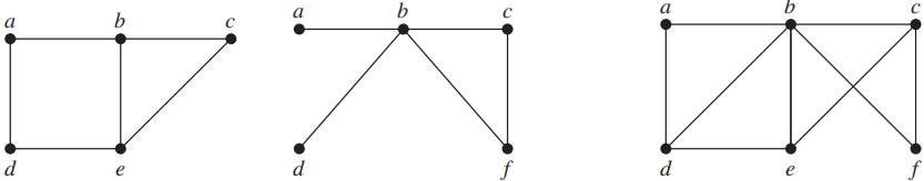
🌰 e.g.
What are the chromatic numbers of the graphs  and
and  ?
?

Solution:
The chromatic number of  is at least 3, because the vertices
  ,
,  , and
, and  must be assigned different colors. To see if
  can be colored with 3 colors, assign red to
  , blue
to  , and green to
  . Then,
  can (and must) be colored red because it is adjacent to
  and
and  , and we have assumed that
  can be colored using only the 3 colors. Furthermore,
  can (and must) be colored green because it is adjacent only to vertices colored red and blue, and
  can (and must) be colored blue because it is adjacent only to vertices colored red and green. Finally,
  can (and must) be colored red because it is adjacent only to vertices colored blue and green. This produces a coloring of
  using exactly 3 colors.
The graph  is made up of the graph
  with an edge connecting a and g. Any attempt to color
  using three colors must follow the same reasoning as that used to color
  , except at the last stage, when all vertices other than
  have been colored. Then, because
  is adjacent (in
  ) to vertices colored red, blue, and green, a fourth color, say brown, needs to be used. Hence,
  has a chromatic number equal to 4.
💡 This solution shows a direct algorithm to find a coloring of a graph by trying to use color that has already been used at each step. Actually, the best algorithms known today for finding the chromatic number of a graph have exponential worst-case time complexity (in the number of vertices of the graph).
📋 The Four Color Theorem
The chromatic number of a planar graph is no greater than four. Or equivalently, any planar map of regions can be depicted using 4 colors so that no two regions that share a positive-length border have the same color.
The four color theorem was originally proposed as a conjecture in 1852. Many fallacious proof with hard-to-find errors were published. It was proved by Haken and Appel used exhaustive computer search in 1976. No proof not relying on computers has yet been found yet until today.
⚠️ The four color theorem applies only to planar graphs. Nonplanar graphs can have arbitrarily large chromatic numbers.
⚙️ Applications of Graph Coloring
- Scheduling Exams: How can the exams at a university be scheduled so that no student has two exams at the same time?
Solution:
This scheduling problem can be solved using a graph model, with vertices representing courses and with an edge between two vertices if there is a common student in the courses they represent. Each time slot for a final exam is represented by a different color. A scheduling of the exams corresponds to a coloring of the associated graph.
- Set up natural habitats of animal in a zoo.
Solution:
Let the vertices of a graph be the animals. Draw an edge between two vertices if the animals they represent cannot be in the same habitat because of their eating habits. A coloring of this graph gives an assignment of habitats.
11. Trees
11.1 Introduction to Trees
A **tree** is a connected simple graph with no simple circuits. A **forest** is a graph that has no simple circuit, but is not connected. Each of the connected components in a forest is a tree.
📋 An undirected graph is a tree if and only if there is a unique simple path between any two of its vertices.
Proof:

- There is a simple path between any two of its vertices because a tree is connected.
- The path is unique because there is no circuit.

- The graph is connected because there are paths between each pair of the vertices.
- The path is unique, so there is no circuit.
A **rooted tree** is a tree in which one vertex has been designated as the **root** and every edge is directed away from the root. An unrooted tree is converted into different rooted trees when different vertices are chosen as the root.
The **parent** of a non-root vertex  is the unique vertex
  with a directed edge from
  to
to  . When
  is the parent of
  ,
,  is called a
 **child** of  . Vertices with the same parent are called
 **siblings**.
The **ancestors** of a non-root vertex are all the vertices in the path from root to this vertex. The **descendants** of vertex  are all the vertices that have
  as an ancestor. The
 **subtree** at vertex  is the subgraph of the tree consisting of vertex
  and its descendants and all edges incident to those descendants. An
 **ordered rooted tree** is a rooted tree where the children of each internal vertex are ordered. In an ordered binary tree, the two possible children of a vertex are called the **left child** and the **right child**, if they exist. The tree rooted at the left child is called the **left subtree**, and that rooted at the right child is called the **right subtree**.
A vertex is called a **leaf** if it has no children. A vertex that have children is called an **internal vertex**.
The **level** of vertex  in a rooted tree is the length of the unique path from the root to
  , and the level of the root is defined to be 0. The
 **height** of a rooted tree is the maximum of the levels of its vertices.
A rooted tree is called a **m-ary tree** if every internal vertex has no more than  children. It is a
 **binary tree** if  . The tree is called a
 **full m-ary tree** if every internal vertex has exactly  children. A rooted m-ary tree of height
  is called
 **balanced** if all its leaves are at levels  or
or  .
.
📋 A tree with  vertices has
  edges.
Proof: ,
,  ,
,  . Any tree must be planar and connected, so
  . Since any tree have no circuits, so
  , so
, so  .
.
🌰 e.g.
A tree has two vertices of degree 2, one vertex of degree 3, three vertices of degree 4. How many leafs does this tree has?
Solution:
Suppose that there are  leaves.
📋 Every tree is a bipartite.
Proof:
Every tree can be colored using two colors. We can choose a root and color it red. Then we color all the vertices at odd levels blue, and all the vertices at even levels red.
📋 A full m-ary tree with  internal vertices contains
  vertices and
  leaves.
Proof:
Every vertex, except the root, is the child of an internal vertex. Since each of the  internal vertices has
  children, there are
  vertices in the tree other than the root. Therefore, the tree contains
  vertices.
📋 A full m-ary tree with  vertices has
  internal vertices and
  leaves.
📋 A full m-ary tree with  leaves has
  vertices and
  internal vertices
📋 For a full binary tree,  .
.
📋 There are at most  leaves in an m-ary tree of height
  . This is proved using MI, from
  to any height with respect to any
  .
.
📋 Corallary
If an m-ary tree of height  has
has  leaves, then
  . If the m-ary tree is full and balanced, then
  .
.
Proof:

Since the tree is balanced. Then each leaf is at level
 or
or  , and since the height is
  , there is at least one leaf at level
  . It follows that
11.2 Applications of Trees
A
**binary search tree (BST)**is an ordered rooted binary tree, each vertex of whom contains a distinct**key value**. The key values in the tree can be compared using “greater than” and “less than”. The key value of each vertex is less than every key value in its right subtree, and greater than every key value in its left subtree.
📋 Construction of BSTsThe first value to be inserted is put into the root.
Thereafter, each value to be inserted begins by comparing itself to the value in the root, moving left it is less, or moving right if it is greater. This continues at each level, until it can be inserted as a new leaf.
Procedure insertion (T: binary search tree, x: item)v:=root of TWhile v≠null and label(v)≠xBeginif x<label(v) thenif left child of v ≠ null thenv:=left child of velseadd new vertex as a left child of v and set v:=nullelseif right child of v ≠ null thenv:=right child of velseadd new vertex as a right child of v and set v:=nullendif root of T = null thenadd a vertex r to the tree and label it with xelse if v is null or label(v)≠x thenlabel new vertex with x and let v be this new vertex{v = location of x}
🌰 e.g.
Insert the elements ‘J’, ‘E’, ‘F’, ‘T’, ‘A’ in that order alphabetically.
Solution:
‘J’ is the first value, so it should be put at the root.
- ‘E’ is less than ‘J’, so it should be the left child of the root.
- ‘F’ is less than ‘J’, so move left; then compare ‘F’ to ‘E’ to find ‘F’ is greater than ‘E’, so ‘F’ should be the right child of ‘E’.
- ‘T’ is greater than ‘J’, so it should be the right child of ‘J’.
- ‘A’ is less than ‘J’ and ‘E’, so it moves left twice and should be the left child of ‘E’.
A rooted tree in which each internal vertex corresponds to a decision, with a subtree at these vertices for each possible outcome of the decision, is called a **decision tree**.
When using bit strings to encode the letters of the English alphabet, using bit strings of different lengths to encode letters can improve coding efficiency. But some method must be used to determine where the bits for each character start and end.
🌰 e.g.
e — 0, a — 1, t — 01. Then 0101 can be “eat”, “tea”, “eaea” or “tt”.
To ensure that no bit string corresponds to more than one sequence of letters, the bit string for a letter must never occur as the first part of the bit string for another letter. Codes with this property are called **prefix codes**.
A system of prefix codes can be constructed using a binary tree. The left edge at each internal vertex is labeled by 0, and the right edge at each internal vertex is labeled by 1. The leaves are labeled by characters which are encoded with the bit string constructed using the labels of the edges in the unique path from the root to the leaves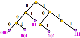
How to produce efficient codes based on the frequencies of occurrences of characters?
General problem:
Tree  has
has  leaves,
  ,
,  ,…,
,…,  are weights representing the frequency of each leaf being used,
  is the length of the code. Let the weight of tree
  be
be  , then
  .
.
For example,
| Letter | a | b | c | d | e | … |
|---|---|---|---|---|---|---|
| Frequency | 82 | 14 | 28 | 38 | 131 | … |
Let  be the length of prefix codes for letter
  , then
Solution:
📋 Huffman Coding
Procedure Huffman (C: symbols ai with frequencies wi, i=1, ... , n)F:=forest of n rooted trees,each consisting of the single vertex ai and assigned weight wiWhile F is not a treebeginReplace the rooted trees T and T’ of least weights from F with w(T) ≥w(T’)with a tree having a new root that has T as its left subtree and T’ as itsright subtree. Label the new edge to T with 0 and the new edge to T’ with 1.Assign w(T) + w(T’) as the weight of the new tree.end{The Huffman coding for the symbol ai is the concatenation of the labels ofthe edges in the unique path from the root to the vertex ai}
🌰 e.g.
Use Huffman coding to encode the following symbols with the frequencies listed: A — 0.08, B — 0.10, C — 0.12, D — 0.15, E — 0.20, F — 0.35. What is the average number of bits used to encode a character?
Solution:

At first, we have a forest of 6 single vertices, and list them in the order of increasing weight. The two vertices with the least weights are A and B, so construct a tree of weight 0.18 using them. List the forest in the order of increasing weight. Then the two vertices with the least weights are C and D, so construct a tree using them. List the forest in the order of increasing weight. Repeat this procedure until the forest become a tree.
11.3 Tree Traversal
A **traversal algorithm** is a procedure for systematically visiting every vertex of an ordered rooted tree. Tree traversals are defined recursively.
Three traversals are named: **preorder**, **inorder**, **postorder**.
📋 Preorder Traversal
Let  be an ordered tree with root
  . If
. If  has only
  , then
  is the preorder traversal of
  . Otherwise, suppose
  ,
,  , … ,
, … ,  are the left to right subtrees at
  . The preorder traversal begins by visiting
  . Then traverses
  in preorder, then traverses
  in preorder, and so on, until
  is traversed in preorder.
procedure preorder (T: ordered rooted tree)r := root of Tlist rfor each child c of r from left to rightT(c) := subtree with c as rootpreorder(T(c))
Preorder traversal of an binary ordered tree:
- Visit the root.
- Visit the left subtree, using preorder.
- Visit the right subtree, using preorder.
🌰 e.g.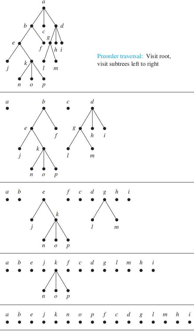
📋 Inorder Traversal
Let  be an ordered tree with root
  . If
. If  has only
  , then
  is the inorder traversal of
  . Otherwise, suppose
  ,
,  , … ,
, … ,  are the left to right subtrees at
  . The inorder traversal begins by traversing
  in inorder. Then visits
  , then traverses
  in inorder, and so on, until
  is traversed in inorder.
procedure inorder (T: ordered rooted tree)r := root of Tif r is a leaf thenlist relsel := first child of r from left to rightT(l) := subtree with l as its rootinorder(T(l))list(r)for each child c of r from left to rightT(c) := subtree with c as rootinorder(T(c))
Inorder traversal of an binary ordered tree:
- Visit the left subtree, using inorder.
- Visit the root.
- Visit the right subtree, using inorder.
🌰 e.g.
📋 Postorder Traversal
Let  be an ordered tree with root
  . If
. If  has only
  , then
  is the postorder traversal of
  . Otherwise, suppose
  ,
,  , … ,
, … ,  are the left to right subtrees at
  . The postorder traversal begins by traversing
  in postorder. Then traverses
  in postorder, until
  is traversed in postorder, finally ends by visiting
  .
.
procedure postordered (T: ordered rooted tree)r := root of Tfor each child c of r from left to rightT(c) := subtree with c as rootpostorder(T(c))list r
Postorder traversal of an binary ordered tree:
- Visit the left subtree, using postorder.
- Visit the right subtree, using postorder.
- Visit the root.
🌰 e.g.
Complicated expressions, such as compound propositions, combinations of sets and arithmetic expressions, can be represented using ordered rooted trees called **expression trees**. A **binary expression tree** is a special kind of binary tree in which each leaf node contains a single operand, each nonleaf node contains a single operator, and the left and right subtrees of an operator node represent subexpressions that must be evaluated before applying the operator at the root of the subtree.
🌰 e.g.
What is the ordered tree that represents the expression  ?
?
Solution:
A binary tree for the expression can be built from the bottom up, as is illustrated here. The higher the priority is, the nearer it should be to the leaves in the expression tree.
An inorder traversal of the expression tree produces the original expression, called the **infix form**(中缀形式), when parentheses are included except for unary operations, which now immediately follow their operands. For example, the infix form we get from the expression tree above is  .
.
The expression obtained by an preorder traversal of the binary tree is said to be in **prefix form**(前缀形式) (Polish notation). For example, the prefix form of the expression tree above is  . In a prefix form, operators precede their operands , parentheses are not needed, as the representation is unambiguous. Prefix expressions are evaluated by working from right to left.
The expression obtained by an postorder traversal of the binary tree is said to be in **postfix form**(后缀形式)(reverse Polish notation 逆波兰记号). For example, the prefix form of the expression tree above is  . Parentheses are not needed as the postfix form is unambiguous, and it evaluate an expression by working from left to right.
11.4-11.5 Spanning Trees & Minimum Spanning Trees
Let  be a simple graph. A
 **spanning tree**(生成树) of  is a subgraph of
  that is a tree containing every vertex of
  . We can find spanning trees of a graph by removing edges from simple circuits(破圈法).
🌰 e.g.
📋 A simple graph is connected if and only if it has a spanning tree.
Proof:
First, suppose that a simple graph  has a spanning tree tree
  .
.  contains every vertex of
  . There is a path in
  between any two of its vertices. Since
  is a subgraph of
  , there is a path in
  between any two of its vertices. Hence
  is connected.
Second, suppose that  is connected. We can find a spanning trees by removing edges from simple circuits of
  .
.
Apart form constructing spanning trees by removing edges, spanning trees can also be built up by successively adding edges. There are two algorithms: depth-first search and breadth-first search.
📋 Depth-First Search(深度优先搜寻)/ Backtracking(回溯)
This procedure forms a rooted tree, and the underlying undirected graph is a spanning tree.
- Arbitrarily choose a vertex of the graph as root.
- From a path starting at this vertex by successively adding edges, where each new edge is incident with the last vertex in the path and a vertex not already in the path.
- Continue adding edges to this path as long as possible.
- If the path goes through all vertices of the graph, the tree consisting of this path is a spanning tree.
- If the path does not go through all vertices, more edges must be added. Move back to the next to last vertex in the path, if possible, form a new path starting at this vertex passing through vertices that were not already visited. If this cannot be done, move back another vertex in the path.
- Repeat this process. ``` procedure DFS(G: connected graph with vertices v1, v2, …, vn) T := tree consisting only of the vertex v1 visit(v1)
procedure visit(v: vertex of G) for each vertex w adjacent to v and not yet in T add vertex w and edge {v,w} to T visit(w)
🌰 e.g.<br />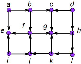<br />What is the output of depth-first search given the graph above as input?<br />Solution:<br />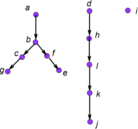<br />📋 Breadth-First Search(广度优先搜寻)1. Arbitrarily choose a vertex of the graph as a root, and add all edges incident to this vertex.2. The new vertices added at this stage become the vertices at level 1 in the spanning tree. Arbitrarily order them.3. For each vertex at level 1, visited in order, add each edge incident to this vertex to the tree as long as it does not produce a simple circuit. Arbitrarily order the children of each vertex at level 1. This produces the vertices at level 2 in the tree.4. Follow the same procedure until all the vertices in the tree have been added.
procedure BFS(G: connected graph with vertices v1, v2, …, vn) T := tree consisting only of the vertex v1 L := empty list visit(v1) put v1 in the list L of unprocessed vertices while L is not empty remove the first vertex, v, from L for each neighbor w of v if w is not in L and not in T then add w to the end of the list L add w and edge {v,w} to T
🌰 e.g.<br />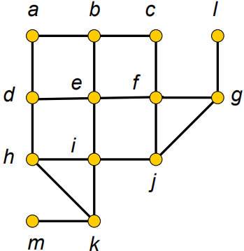<br />Use a breadth-first search to find a spanning tree for the graph above.<br />Solution:<br />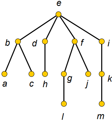<br />There are problems that can be solved only by performing an exhaustive search of all possible solutions. One way to search systematically for a solution is to build a decision tree using `**backtracking scheme**`(回溯法), where each internal vertex represents a decision and each leaf a possible solution.<br />A `**minimum spanning tree**` in a connected weighted graph is a spanning tree that has the smallest possible sum of weights of its edges.<br />Two algorithms for constructing minimum spanning trees: Prim's algorithm and Kruskal's algorithm. These two algorithms are examples of greedy algorithms, both proceed by successively adding edges of smallest weight from those edges with a specified property that have not already been used.<br />📋 Prim's Algorithm
Procedure Prim (G: weighted connected undirected graph with n vertices) T:= a minimum-weight edge for i:= 1 to n-2 begin e:= an edge of minimum weight incident to a vertex in T and not forming a simple circuit in T if added to T. T:= T with e added end {T is a minimum spanning tree of G}
📋 Kruskal's Algorithm(最简单)
Procedure Kruskal (G: weighted connected undirected graph with n vertices)
T:= empty graph
for i:= 1 to n-1
begin
e:= any edge in G with smallest weight that does not
form a simple circuit when added to T
T:= T with e added
end {T is a minimum spanning tree of G}
```
🌰 e.g.
Find a minimum spanning tree in the weighted graph.
Solution:
| Prim’s algorithm | ||
|---|---|---|
| Choice | Edge | Cost |
| 1 | BE | 700 |
| 2 | EC | 800 |
| 3 | BA | 1200 |
| 4 | AD | 900 |
| Total | 3600 |
| Kruskal’s algorithm | ||
|---|---|---|
| Choice | Edge | Cost |
| 1 | BE | 700 |
| 2 | EC | 800 |
| 3 | AD | 900 |
| 4 | AB | 1200 |
| Total | 3600 |

若有收获,就点个赞吧
0 人点赞
