tidymodels-exercise-01
liyue
Last compiled on 04 七月, 2021
探索数据
library(tidyverse)## -- Attaching packages --------------------------------------- tidyverse 1.3.1 --## v ggplot2 3.3.3 v purrr 0.3.4## v tibble 3.1.1 v dplyr 1.0.6## v tidyr 1.1.3 v stringr 1.4.0## v readr 1.4.0 v forcats 0.5.1## -- Conflicts ------------------------------------------ tidyverse_conflicts() --## x dplyr::filter() masks stats::filter()## x dplyr::lag() masks stats::lag()
首先读取数据,在这个出勤率的数据中,weekly_attendance是需要预测的结果。
attendance <- read_csv("../datasets/tidytuesday/data/2020/2020-02-04/attendance.csv")#### -- Column specification --------------------------------------------------------## cols(## team = col_character(),## team_name = col_character(),## year = col_double(),## total = col_double(),## home = col_double(),## away = col_double(),## week = col_double(),## weekly_attendance = col_double()## )standings <- read_csv("../datasets/tidytuesday/data/2020/2020-02-04/standings.csv")#### -- Column specification --------------------------------------------------------## cols(## team = col_character(),## team_name = col_character(),## year = col_double(),## wins = col_double(),## loss = col_double(),## points_for = col_double(),## points_against = col_double(),## points_differential = col_double(),## margin_of_victory = col_double(),## strength_of_schedule = col_double(),## simple_rating = col_double(),## offensive_ranking = col_double(),## defensive_ranking = col_double(),## playoffs = col_character(),## sb_winner = col_character()## )attendance_joined <- attendance %>%left_join(standings,by = c("year", "team_name", "team"))attendance_joined## # A tibble: 10,846 x 20## team team_name year total home away week weekly_attendan~ wins loss## <chr> <chr> <dbl> <dbl> <dbl> <dbl> <dbl> <dbl> <dbl> <dbl>## 1 Ariz~ Cardinals 2000 893926 387475 506451 1 77434 3 13## 2 Ariz~ Cardinals 2000 893926 387475 506451 2 66009 3 13## 3 Ariz~ Cardinals 2000 893926 387475 506451 3 NA 3 13## 4 Ariz~ Cardinals 2000 893926 387475 506451 4 71801 3 13## 5 Ariz~ Cardinals 2000 893926 387475 506451 5 66985 3 13## 6 Ariz~ Cardinals 2000 893926 387475 506451 6 44296 3 13## 7 Ariz~ Cardinals 2000 893926 387475 506451 7 38293 3 13## 8 Ariz~ Cardinals 2000 893926 387475 506451 8 62981 3 13## 9 Ariz~ Cardinals 2000 893926 387475 506451 9 35286 3 13## 10 Ariz~ Cardinals 2000 893926 387475 506451 10 52244 3 13## # ... with 10,836 more rows, and 10 more variables: points_for <dbl>,## # points_against <dbl>, points_differential <dbl>, margin_of_victory <dbl>,## # strength_of_schedule <dbl>, simple_rating <dbl>, offensive_ranking <dbl>,## # defensive_ranking <dbl>, playoffs <chr>, sb_winner <chr>
看看不同队伍之间出勤率的差别,以及有无季后赛的影响?
attendance_joined %>%filter(!is.na(weekly_attendance)) %>%ggplot(., aes(fct_reorder(team_name, weekly_attendance), weekly_attendance, fill = playoffs)) +geom_boxplot(outlier.alpha = 0.3) +labs(fill = NULL, x = NULL, y = "weekly attendance") +theme(legend.position = "bottom") +theme_bw() +coord_flip()

不同的周对出勤率有没有影响?
attendance_joined %>%mutate(week = factor(week)) %>%ggplot(., aes(week, weekly_attendance, fill = week)) +geom_boxplot(show.legend = F, outlier.alpha = 0.3) +labs(x = "week", y = "weekly attendance")+theme_bw()

建立模型
首先删除结果变量(weekly attendance)是NA的行,并选择想作为预测变量的列。
attendance_df <- attendance_joined %>%filter(!is.na(weekly_attendance)) %>%select(weekly_attendance, team_name, year, week, margin_of_victory, strength_of_schedule, playoffs)attendance_df## # A tibble: 10,208 x 7## weekly_attendance team_name year week margin_of_victory strength_of_schedu~## <dbl> <chr> <dbl> <dbl> <dbl> <dbl>## 1 77434 Cardinals 2000 1 -14.6 -0.7## 2 66009 Cardinals 2000 2 -14.6 -0.7## 3 71801 Cardinals 2000 4 -14.6 -0.7## 4 66985 Cardinals 2000 5 -14.6 -0.7## 5 44296 Cardinals 2000 6 -14.6 -0.7## 6 38293 Cardinals 2000 7 -14.6 -0.7## 7 62981 Cardinals 2000 8 -14.6 -0.7## 8 35286 Cardinals 2000 9 -14.6 -0.7## 9 52244 Cardinals 2000 10 -14.6 -0.7## 10 64223 Cardinals 2000 11 -14.6 -0.7## # ... with 10,198 more rows, and 1 more variable: playoffs <chr>
分割数据
library(tidymodels)## -- Attaching packages -------------------------------------- tidymodels 0.1.3 --## v broom 0.7.6 v rsample 0.0.9## v dials 0.0.9 v tune 0.1.5## v infer 0.5.4 v workflows 0.2.2## v modeldata 0.1.0 v workflowsets 0.0.2## v parsnip 0.1.5 v yardstick 0.0.8## v recipes 0.1.16## -- Conflicts ----------------------------------------- tidymodels_conflicts() --## x scales::discard() masks purrr::discard()## x dplyr::filter() masks stats::filter()## x recipes::fixed() masks stringr::fixed()## x dplyr::lag() masks stats::lag()## x yardstick::spec() masks readr::spec()## x recipes::step() masks stats::step()## * Use tidymodels_prefer() to resolve common conflicts.set.seed(123)attendance_split <- attendance_df %>%initial_split(strata = playoffs)nfl_train <- training(attendance_split)nfl_test <- testing(attendance_split)
建立一个线性回归模型
lm_spec <- linear_reg() %>% set_engine("lm")lm_fit <- lm_spec %>% fit(weekly_attendance ~ ., data = nfl_train)lm_fit## parsnip model object#### Fit time: 31ms#### Call:## stats::lm(formula = weekly_attendance ~ ., data = data)#### Coefficients:## (Intercept) team_nameBears team_nameBengals## -104175.10 -3112.97 -5261.15## team_nameBills team_nameBroncos team_nameBrowns## -465.98 3157.94 -248.44## team_nameBuccaneers team_nameCardinals team_nameChargers## -3585.25 -6652.83 -5165.30## team_nameChiefs team_nameColts team_nameCowboys## 1314.75 -3654.27 6141.39## team_nameDolphins team_nameEagles team_nameFalcons## 312.73 1345.57 -398.50## team_nameGiants team_nameJaguars team_nameJets## 5637.37 -3189.05 3914.46## team_nameLions team_namePackers team_namePanthers## -3190.57 1181.02 1886.74## team_namePatriots team_nameRaiders team_nameRams## -262.90 -5526.03 -2582.71## team_nameRavens team_nameRedskins team_nameSaints## -501.41 6537.25 130.27## team_nameSeahawks team_nameSteelers team_nameTexans## -1962.10 -3343.01 85.38## team_nameTitans team_nameVikings year## -1101.85 -2633.05 86.13## week margin_of_victory strength_of_schedule## -68.54 127.51 238.26## playoffsPlayoffs## -171.49
建立一个随机森林回归模型
rf_spec <- rand_forest(mode = "regression") %>% set_engine("ranger")rf_fit <- rf_spec %>% fit(weekly_attendance ~ ., data = nfl_train)rf_fit## parsnip model object#### Fit time: 4.8s## Ranger result#### Call:## ranger::ranger(x = maybe_data_frame(x), y = y, num.threads = 1, verbose = FALSE, seed = sample.int(10^5, 1))#### Type: Regression## Number of trees: 500## Sample size: 7656## Number of independent variables: 6## Mtry: 2## Target node size: 5## Variable importance mode: none## Splitrule: variance## OOB prediction error (MSE): 74791027## R squared (OOB): 0.06967497
评价模型
使用测试集评价模型
# 下面这段合并结果的代码可以用于很多模型,值得学习results_train <- lm_fit %>%predict(new_data = nfl_train) %>%mutate(truth = nfl_train$weekly_attendance,model = "lm") %>%bind_rows(rf_fit %>%predict(new_data = nfl_train) %>%mutate(truth = nfl_train$weekly_attendance,model = "rf"))results_train## # A tibble: 15,312 x 3## .pred truth model## <dbl> <dbl> <chr>## 1 59263. 66009 lm## 2 59126. 71801 lm## 3 59058. 66985 lm## 4 58989. 44296 lm## 5 58920. 38293 lm## 6 58852. 62981 lm## 7 58783. 35286 lm## 8 58715. 52244 lm## 9 58646. 64223 lm## 10 58578. 65356 lm## # ... with 15,302 more rowsresults_test <- lm_fit %>%predict(new_data = nfl_test) %>%mutate(truth = nfl_test$weekly_attendance,model = "lm") %>%bind_rows(rf_fit %>%predict(new_data = nfl_test)%>%mutate(truth = nfl_test$weekly_attendance,model = "rf"))results_test## # A tibble: 5,104 x 3## .pred truth model## <dbl> <dbl> <chr>## 1 59332. 77434 lm## 2 65999. 74309 lm## 3 65656. 64900 lm## 4 68015. 68843 lm## 5 67809. 73018 lm## 6 67672. 83252 lm## 7 67261. 68361 lm## 8 67654. 77884 lm## 9 67174. 60292 lm## 10 66968. 65546 lm## # ... with 5,094 more rows
用rmse看看效果
results_train %>%group_by(model) %>%rmse(truth = truth, estimate = .pred)## # A tibble: 2 x 4## model .metric .estimator .estimate## <chr> <chr> <chr> <dbl>## 1 lm rmse standard 8267.## 2 rf rmse standard 6090.results_test %>%group_by(model) %>%rmse(truth = truth, estimate = .pred)## # A tibble: 2 x 4## model .metric .estimator .estimate## <chr> <chr> <chr> <dbl>## 1 lm rmse standard 8471.## 2 rf rmse standard 8639.
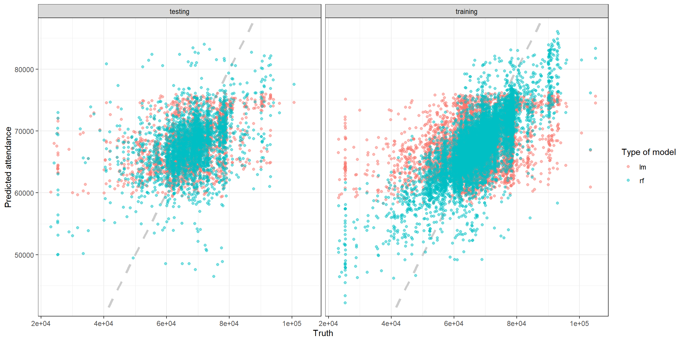
可视化结果
results_test %>%mutate(train = "testing") %>%bind_rows(results_train %>%mutate(train = "training")) %>%ggplot(aes(truth, .pred, color = model)) +geom_abline(lty = 2, color = "gray80", size = 1.5) +geom_point(alpha = 0.5) +facet_wrap(~train) +labs(x = "Truth",y = "Predicted attendance",color = "Type of model")+theme_bw()
使用交叉验证再试一次
set.seed(123)nfl_folds <- vfold_cv(nfl_train, strata = playoffs)rf_res <- fit_resamples(rf_spec,weekly_attendance ~ .,nfl_folds,control = control_resamples(save_pred = TRUE))rf_res %>%collect_metrics()## # A tibble: 2 x 6## .metric .estimator mean n std_err .config## <chr> <chr> <dbl> <int> <dbl> <chr>## 1 rmse standard 8616. 10 127. Preprocessor1_Model1## 2 rsq standard 0.112 10 0.0112 Preprocessor1_Model1
可视化结果
rf_res %>%unnest(.predictions) %>%ggplot(aes(weekly_attendance, .pred, color = id)) +geom_abline(lty = 2, color = "gray80", size = 1.5) +geom_point(alpha = 0.5) +labs(x = "Truth",y = "Predicted game attendance",color = NULL)+theme_bw()


若有收获,就点个赞吧
0 人点赞
