应用预测建模 - 应用预测建模2：过度拟合和模型调优 - 《R语言机器学习》

基本概念
计算

基本概念

过拟合

在模型学习数据普遍化模式的过程中，它还学习了每个样本特有的噪音特征，这样的模型称为过拟合。
过拟合的模型可能在原数据集上的表现非常好，但是泛化能力很差，也就是换一个数据集表现就很差，这就是由于过拟合导致的。

模型调优

几乎所有的预测模型方法都含有调优参数，用现有的数据来调整这些参数，从而给出最好的预测，这个过程称为模型调优。

数据分割

数据量较小时应避免划分测试集。
如果某类的样本量明显少于其他类，那么简单的随机划分会导致训练集和测试集结果大相径庭，应使用分层随机抽样法

重抽样技术

K折交叉验证
广义交叉验证
重复训练/测试集划分
Bootstrap方法

数据划分建议

样本量较少，笔者建议使用10折交叉验证
如果目标不是得到最好的模型表现的估计，而是在几个不同的模型中进行选择，那么最好使用Bootstrap方法

计算

## 加载R包和数据
library(AppliedPredictiveModeling)
data(twoClassData)
str(predictors)
## 'data.frame':    208 obs. of  2 variables:
##  $ PredictorA: num  0.158 0.655 0.706 0.199 0.395 ...
##  $ PredictorB: num  0.1609 0.4918 0.6333 0.0881 0.4152 ...
str(classes)
##  Factor w/ 2 levels "Class1","Class2": 2 2 2 2 2 2 2 2 2 2 ...
set.seed(1)

# 划分数据集
library(caret)
## 载入需要的程辑包：lattice
## 载入需要的程辑包：ggplot2
trainingRows <- createDataPartition(classes, p = 0.8, list = F) # 也可进行分层抽样
head(trainingRows)
##      Resample1
## [1,]         1
## [2,]         2
## [3,]         3
## [4,]         7
## [5,]         8
## [6,]         9

变为训练集和测试集：

trainPredictors <- predictors[trainingRows, ]
trainClasses <- classes[trainingRows]
testPredictors <- predictors[-trainingRows, ]
testClasses <- classes[-trainingRows]
str(trainPredictors)
## 'data.frame':    167 obs. of  2 variables:
##  $ PredictorA: num  0.1582 0.6552 0.706 0.0658 0.3086 ...
##  $ PredictorB: num  0.161 0.492 0.633 0.179 0.28 ...
str(testPredictors)
## 'data.frame':    41 obs. of  2 variables:
##  $ PredictorA: num  0.1992 0.3952 0.425 0.0847 0.2909 ...
##  $ PredictorB: num  0.0881 0.4152 0.2988 0.0548 0.3021 ...

## 重抽样
set.seed(1)
repeatedSplits <- createDataPartition(trainClasses, p = 0.8, times = 3)
str(repeatedSplits)
## List of 3
##  $ Resample1: int [1:135] 1 2 3 4 6 7 9 10 11 12 ...
##  $ Resample2: int [1:135] 1 2 3 4 5 6 7 9 10 11 ...
##  $ Resample3: int [1:135] 1 2 3 4 5 7 8 9 11 12 ...

## K折交叉验证
set.seed(1)
cvSplits <- createFolds(trainClasses, k = 10, returnTrain = T)
str(cvSplits)
## List of 10
##  $ Fold01: int [1:150] 1 2 4 5 6 7 8 10 11 13 ...
##  $ Fold02: int [1:150] 1 2 3 4 6 7 8 9 10 11 ...
##  $ Fold03: int [1:150] 1 3 4 5 6 7 8 9 10 11 ...
##  $ Fold04: int [1:150] 1 2 3 4 5 6 7 8 9 10 ...
##  $ Fold05: int [1:150] 2 3 4 5 6 7 8 9 10 11 ...
##  $ Fold06: int [1:150] 1 2 3 4 5 6 7 8 9 11 ...
##  $ Fold07: int [1:150] 1 2 3 4 5 6 7 9 10 12 ...
##  $ Fold08: int [1:151] 1 2 3 4 5 6 8 9 10 11 ...
##  $ Fold09: int [1:151] 1 2 3 5 6 7 8 9 10 11 ...
##  $ Fold10: int [1:151] 1 2 3 4 5 7 8 9 10 11 ...
fold1 <- cvSplits[[1]] # 第一折的行号
cvPredictors1 <- trainPredictors[fold1, ] # 得到第一份90%的样本
cvClass1 <- trainClasses[fold1]
nrow(trainPredictors)
## [1] 167
nrow(cvPredictors1)
## [1] 150

## R基础建模
## 训练
trainPredictors <- as.matrix(trainPredictors)
knnFit <- knn3(x = trainPredictors, y = trainClasses, k = 5)
knnFit
## 5-nearest neighbor model
## Training set outcome distribution:
## 
## Class1 Class2 
##     89     78
## 预测
testPredictions <- predict(knnFit, newdata = testPredictors, type = "class")
head(testPredictions)
## [1] Class2 Class1 Class1 Class2 Class1 Class2
## Levels: Class1 Class2
str(testPredictions)
##  Factor w/ 2 levels "Class1","Class2": 2 1 1 2 1 2 2 1 2 2 ...

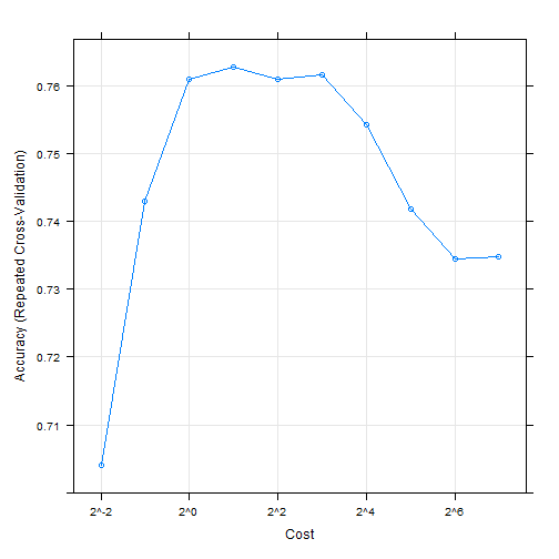
## 决定调优参数
library(caret)
data("GermanCredit")
set.seed(1056)
svmFit <- train(Class ~., 
                data = GermanCredit,
                method = "svmRadial")
## 进行预处理，并使用重复5折交叉验证
set.seed(1056)
svmfit <- train(Class ~., 
                data = GermanCredit,
                method = "svmRadial",
                preProc = c("center" ,"scale"),
                tuneLength = 10,
                trControl = trainControl(method = "repeatedcv", repeats = 5)
                ) # 其实这个函数我感觉比现在的tidymodels和mlr3的写法都要简洁...
svmfit
## Support Vector Machines with Radial Basis Function Kernel 
## 
## 1000 samples
##   61 predictor
##    2 classes: 'Bad', 'Good' 
## 
## Pre-processing: centered (61), scaled (61) 
## Resampling: Cross-Validated (10 fold, repeated 5 times) 
## Summary of sample sizes: 900, 900, 900, 900, 900, 900, ... 
## Resampling results across tuning parameters:
## 
##   C       Accuracy  Kappa     
##     0.25  0.7040    0.01934723
##     0.50  0.7430    0.24527603
##     1.00  0.7610    0.35046362
##     2.00  0.7628    0.38285072
##     4.00  0.7610    0.39239970
##     8.00  0.7616    0.40357861
##    16.00  0.7542    0.39860268
##    32.00  0.7418    0.37677389
##    64.00  0.7344    0.36165095
##   128.00  0.7348    0.36361822
## 
## Tuning parameter 'sigma' was held constant at a value of 0.009718427
## Accuracy was used to select the optimal model using the largest value.
## The final values used for the model were sigma = 0.009718427 and C = 2.
plot(svmfit, scales = list(x=list(log = 2)))

应用预测建模2：过度拟合和模型调优 - 图1

## 比较模型
set.seed(1056)
logistic <- train(Class ~., 
                  data = GermanCredit,
                  method = "glm",
                  trControl = trainControl(method = "repeatedcv", repeats = 5)
                  )
logistic
## Generalized Linear Model 
## 
## 1000 samples
##   61 predictor
##    2 classes: 'Bad', 'Good' 
## 
## No pre-processing
## Resampling: Cross-Validated (10 fold, repeated 5 times) 
## Summary of sample sizes: 900, 900, 900, 900, 900, 900, ... 
## Resampling results:
## 
##   Accuracy  Kappa    
##   0.749     0.3661277
resamp <- resamples(list(svm = svmfit, logi = logistic))
summary(resamp)
## 
## Call:
## summary.resamples(object = resamp)
## 
## Models: svm, logi 
## Number of resamples: 50 
## 
## Accuracy 
##      Min. 1st Qu. Median   Mean 3rd Qu. Max. NA's
## svm  0.69  0.7425   0.77 0.7628  0.7800 0.84    0
## logi 0.65  0.7200   0.75 0.7490  0.7775 0.88    0
## 
## Kappa 
##           Min.   1st Qu.    Median      Mean   3rd Qu.      Max. NA's
## svm  0.1944444 0.3385694 0.3882979 0.3828507 0.4293478 0.5959596    0
## logi 0.1581633 0.2993889 0.3779762 0.3661277 0.4240132 0.7029703    0
summary(diff(resamp))
## 
## Call:
## summary.diff.resamples(object = diff(resamp))
## 
## p-value adjustment: bonferroni 
## Upper diagonal: estimates of the difference
## Lower diagonal: p-value for H0: difference = 0
## 
## Accuracy 
##      svm       logi  
## svm            0.0138
## logi 0.0002436       
## 
## Kappa 
##      svm     logi   
## svm          0.01672
## logi 0.07449