时间序列分析实践

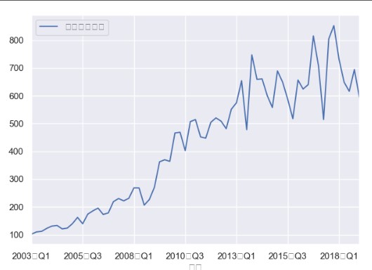
题目：03年到19年第一季度分季度的数据，13年之前只有传统汽车的销量，13年之后是传统汽车+新能源汽车的销量，需要预测未来三期传统汽车的销量～

import pandas as pd
import matplotlib.pyplot as plt
data = pd.read_excel("C:\orange_credit\crdt\时序数据.xlsx", sheet_name='Sheet2', index_col=u'日期')
#先画出日期和传统车型销量的图形，可以判断是非平稳的
data.plot()
plt.show()

所使用的源代码：

def test_stationarity(timeseries):
    # 滚动平均
    rolmean = pd.rolling_mean(timeseries, window=12)
    rolstd = pd.rolling_std(timeseries, window=12)
    ts_diff = timeseries - timeseries.shift()
    orig = timeseries.plot(color='blue', label='Original')
    mean = rolmean.plot(color='red', label='Rolling Mean')
    std = rolstd.plot(color='black', label='Rolling Std')
    diff = ts_diff.plot(color='green', label='Diff 1')
    plt.legend(loc='best')
    plt.title('Rolling Mean & Standard Deviation')
    plt.show(block=False)
    # adf检验
    print('Result of Dickry-Fuller test')
    dftest = adfuller(timeseries, autolag='AIC')
    dfoutput = pd.Series(dftest[0:4], index=['Test Statistic', 'p-value', '#Lags Used', 'Number of observations Used'])
    for key, value in dftest[4].items():
        dfoutput['Critical value(%s)' % key] = value
    print(dfoutput)
#test_stationarity(ts)
def test_stationarity(timeseries):
    # 滚动平均#差分#标准差
    rolmean = pd.rolling_mean(timeseries, window=12)
    ts_diff = timeseries - timeseries.shift()
    rolstd = pd.rolling_std(timeseries, window=12)
    orig = timeseries.plot(color='blue', label='Original')
    mean = rolmean.plot(color='red', label='Rolling 12 Mean')
    std = rolstd.plot(color='black', label='Rolling 12 Std')
    diff = ts_diff.plot(color='green', label='Diff 1')
    plt.legend(loc='best')
    plt.title('Rolling Mean and Standard Deviation and Diff 1')
    l1 = plt.axhline(y=0, linewidth=1, color='yellow')
    plt.show(block=False)
    # adf--AIC检验
    print('Result of Augment Dickry-Fuller test--AIC')
    dftest = adfuller(timeseries, autolag='AIC')
    dfoutput = pd.Series(dftest[0:4], index=['Test Statistic', 'p-value', 'Lags Used',
                                             'Number of observations Used'])
    for key, value in dftest[4].items():
        dfoutput['Critical value(%s)' % key] = value
    print(dfoutput)
    # adf--BIC检验
    print('-------------------------------------------')
    print('Result of Augment Dickry-Fuller test--BIC')
    dftest = adfuller(timeseries, autolag='BIC')
    dfoutput = pd.Series(dftest[0:4], index=['Test Statistic', 'p-value', 'Lags Used',
                                             'Number of observations Used'])
    for key, value in dftest[4].items():
        dfoutput['Critical value(%s)' % key] = value
    print(dfoutput)
test_stationarity(ts)
# 不取对数，直接减掉趋势
ts.index = ts.index.to_timestamp()
moving_avg = pd.rolling_mean(ts, 12)
plt.plot(ts)
plt.plot(moving_avg, color='red')
plt.show()
ts_moving_avg_diff = ts - moving_avg
ts_moving_avg_diff.head(12)
# 再一次确定平稳性
ts_moving_avg_diff.dropna(inplace=True)
test_stationarity(ts_moving_avg_diff)
expwighted_avg = pd.ewma(ts, halflife=12)
plt.plot(ts)
plt.plot(expwighted_avg, color='red')
plt.show()
# 减掉指数平滑法
ts_ewma_diff = ts - expwighted_avg
test_stationarity(ts_ewma_diff)
# 差分法1
ts_diff = ts - ts.shift()
plt.plot(ts_diff)
plt.show()
# 差分方法2
fig = plt.figure(figsize=(12, 8))
ax1 = fig.add_subplot(111)
diff1 = ts.diff(1)
# diff2 = diff1.diff(1)
diff1.plot(ax=ax1)
plt.show()
ts_diff.dropna(inplace=True)
test_stationarity(ts_diff)
plt.show()
from statsmodels.tsa.seasonal import seasonal_decompose
decomposition = seasonal_decompose(ts)
trend = decomposition.trend
seasonal = decomposition.seasonal
residual = decomposition.resid
plt.subplot(411)
plt.plot(ts, label='Original')
plt.legend(loc='best')
plt.subplot(412)
plt.plot(trend, label='Trend')
plt.legend(loc='best')
plt.subplot(413)
plt.plot(seasonal, label='Seasonality')
plt.legend(loc='best')
plt.subplot(414)
plt.plot(residual, label='Residuals')
plt.legend(loc='best')
plt.tight_layout()
plt.show()
# 直接对残差进行分析，我们检查残差的稳定性
ts_decompose = residual
ts_decompose.dropna(inplace=True)
test_stationarity(ts_decompose)
fig = plt.figure(figsize=(12, 8))
ax1 = fig.add_subplot(211)
fig = sm.graphics.tsa.plot_acf(ts_diff, lags=20, ax=ax1)
ax1.xaxis.set_ticks_position('bottom')
fig.tight_layout();
ax2 = fig.add_subplot(212)
fig = sm.graphics.tsa.plot_pacf(ts_diff, lags=20, ax=ax2)
ax2.xaxis.set_ticks_position('bottom')
plt.show()
fig.tight_layout();
# trend
fig = plt.figure(figsize=(12, 8))
ax1 = fig.add_subplot(211)
fig = sm.graphics.tsa.plot_acf(trend, lags=20, ax=ax1)
ax1.xaxis.set_ticks_position('bottom')
fig.tight_layout();
ax2 = fig.add_subplot(212)
fig = sm.graphics.tsa.plot_pacf(trend, lags=20, ax=ax2)
ax2.xaxis.set_ticks_position('bottom')
plt.show()
fig.tight_layout();
# seasonal
fig = plt.figure(figsize=(12, 8))
ax1 = fig.add_subplot(211)
fig = sm.graphics.tsa.plot_acf(seasonal, lags=20, ax=ax1)
ax1.xaxis.set_ticks_position('bottom')
fig.tight_layout();
ax2 = fig.add_subplot(212)
fig = sm.graphics.tsa.plot_pacf(seasonal, lags=20, ax=ax2)
ax2.xaxis.set_ticks_position('bottom')
plt.show()
fig.tight_layout();
import itertools
# Define the p, d and q parameters to take any value between 0 and 2
p = d = q = range(0, 3)
# Generate all different combinations of p, q and q triplets
pdq = list(itertools.product(p, d, q))
print('p,d,q', pdq, '\n')
for param in pdq:
    try:
        model = ARIMA(ts_diff, order=param)
        # model=ARIMA(ts_log,order=(2,1,2))
        result_ARIMA = model.fit(disp=-1)
        print('ARIMA{}-- AIC:{} -- BIC:{} --HQIC:{}'.format(
            param, result_ARIMA.aic, result_ARIMA.bic, result_ARIMA.hqic))
    except:
        continue
# AR model
model = ARIMA(seasonal, order=(2, 0, 0))
result_AR = model.fit(disp=-1)
plt.plot(seasonal)
plt.plot(result_AR.fittedvalues, color='blue')
plt.title('RSS:%.4f' % sum(result_AR.fittedvalues - seasonal) ** 2)
plt.show()
# AR model
model = ARIMA(ts_diff, order=(2, 0, 0))
result_AR = model.fit(disp=-1)
plt.plot(ts_diff)
plt.plot(result_AR.fittedvalues, color='blue')
plt.title('RSS:%.4f' % sum(result_AR.fittedvalues - ts_diff) ** 2)
plt.show()
# MA model
model = ARIMA(ts_diff, order=(0, 0, 2))
result_MA = model.fit(disp=-1)
plt.plot(ts_diff)
plt.plot(result_MA.fittedvalues, color='blue')
plt.title('RSS:%.4f' % sum(result_MA.fittedvalues - ts_diff) ** 2)
plt.show()
# ARIMA 将两个结合起来  效果更好
# warnings.filterwarnings("ignore") # specify to ignore warning messages
import itertools
# Define the p, d and q parameters to take any value between 0 and 2
p = d = q = range(0, 3)
# Generate all different combinations of p, q and q triplets
pdq = list(itertools.product(p, d, q))
print('p,d,q', pdq, '\n')
for param in pdq:
    try:
        model = ARIMA(ts_diff, order=param)
        # model=ARIMA(ts_log,order=(2,1,2))
        result_ARIMA = model.fit(disp=-1)
        print('ARIMA{}- AIC:{} - BIC:{} - HQIC:{}'.format(param, result_ARIMA.aic, result_ARIMA.bic, result_ARIMA.hqic))
    except:
        continue
# MA
# model=ARIMA(ts_log,order=(2,1,2))
model = ARIMA(ts_diff, order=(0, 0, 2))
result_ARIMA_diff = model.fit(disp=-1)
plt.plot(ts_diff)
plt.plot(result_ARIMA_diff.fittedvalues, color='blue')
plt.title('RSS:%.4f' % sum(result_ARIMA_diff.fittedvalues - ts_diff) ** 2)
plt.show()
# ARMA
# model=ARIMA(ts_log,order=(2,1,2))
model = ARIMA(ts_diff, order=(1, 0, 2))
result_ARIMA_diff = model.fit(disp=-1)
plt.plot(ts_diff)
plt.plot(result_ARIMA_diff.fittedvalues, color='blue')
plt.title('RSS:%.4f' % sum(result_ARIMA_diff.fittedvalues - ts_diff) ** 2)
plt.show()
# 检验部分
fig = plt.figure(figsize=(12, 8))
ax1 = fig.add_subplot(211)
fig = sm.graphics.tsa.plot_acf(result_ARIMA_diff.resid.values.squeeze(), lags=40, ax=ax1)
ax2 = fig.add_subplot(212)
fig = sm.graphics.tsa.plot_pacf(result_ARIMA_diff.resid, lags=40, ax=ax2)
plt.show()
import statsmodels.api as sm
print(sm.stats.durbin_watson(result_ARIMA_diff.resid.values))
# 2附近即不存在一阶自相关
# 检验结果是2.02424743723，说明不存在自相关性。
resid = result_ARIMA_diff.resid  # 残差
fig = plt.figure(figsize=(12, 8))
ax = fig.add_subplot(111)
fig = qqplot(resid, line='q', ax=ax, fit=True)
plt.show()
# LJ检验
r, q, p = sm.tsa.acf(result_ARIMA_diff.resid.values.squeeze(), qstat=True)
data = np.c_[range(1, 41), r[1:], q, p]
table = pd.DataFrame(data, columns=['lag', "AC", "Q", "Prob(>Q)"])
print(table.set_index('lag'))
# model=ARIMA(ts_log,order=(2,1,2))
model_results = ARIMA(ts_diff, order=(1, 0, 2))
result_ARIMA = model_results.fit(disp=-1)
# fig, ax = plt.subplots(figsize=(12, 8))
# ax = ts.ix['1962':].plot(ax=ax)
# fig = result_ARIMA.plot_predict('1976-01', '1976-12', dynamic=True, ax=ax, plot_insample=False)
result_ARIMA.plot_predict()
result_ARIMA.forecast()
plt.show()
predictions_ARIMA_diff = pd.Series(result_ARIMA_diff.fittedvalues, copy=True)
print(predictions_ARIMA_diff.head())
print('------------------------')
predictions_ARIMA_diff_cumsum = predictions_ARIMA_diff.cumsum()
print(predictions_ARIMA_diff_cumsum.head())
predictions_ARIMA = pd.Series(ts.ix[0], index=ts.index)
predictions_ARIMA_cus = predictions_ARIMA.add(predictions_ARIMA_diff_cumsum, fill_value=0)
predictions_ARIMA_cus.head()
plt.plot(ts)
plt.plot(predictions_ARIMA_cus)
plt.title('RMSE: %.4f' % np.sqrt(sum((predictions_ARIMA_cus - ts) ** 2) / len(ts)))
plt.show()
# 对的--加上了预测的值
predict_dta = result_ARIMA_diff.predict('1976-01', '1976-12', dynamic=True)
AA = predictions_ARIMA_diff.append(predict_dta)
predictions_ARIMA = pd.Series(ts.ix[0], index=pd.period_range('196202', '197612', freq='M'))
AA.index = pd.period_range('196202', '197612', freq='M')
predictions_ARIMA2 = predictions_ARIMA.add(AA.cumsum(), fill_value=0)
ts.plot()
predictions_ARIMA2.plot()
plt.show()