介绍
官方文档:
https://bioconductor.org/packages/release/bioc/vignettes/SingleR/inst/doc/SingleR.html
SingleR能够基于现有的参考数据集对单细胞分析中获取的cluster进行自动注释。(只能对人和小鼠的数据进行注释,因为暂时只有人和小鼠的参考数据集)
SingleR is an automatic annotation method for single-cell RNA sequencing (scRNAseq) data (Aran et al. 2019). Given a reference dataset of samples (single-cell or bulk) with known labels, it labels new cells from a test dataset based on similarity to the reference set. Specifically, for each test cell:
- We compute the Spearman correlation between its expression profile and that of each reference sample. This is done across the union of marker genes identified between all pairs of labels.
- We define the per-label score as a fixed quantile (by default, 0.8) of the distribution of correlations.
- We repeat this for all labels and we take the label with the highest score as the annotation for this cell.
- We optionally perform a fine-tuning step:
- The reference dataset is subsetted to only include labels with scores close to the maximum.
- Scores are recomputed using only marker genes for the subset of labels.
- This is iterated until one label remains.
R包安装
options("repos" = c(CRAN="http://mirrors.cloud.tencent.com/CRAN/"))options(BioC_mirror="http://mirrors.cloud.tencent.com/bioconductor")BiocManager::install("SingleR")
参考数据集的获取
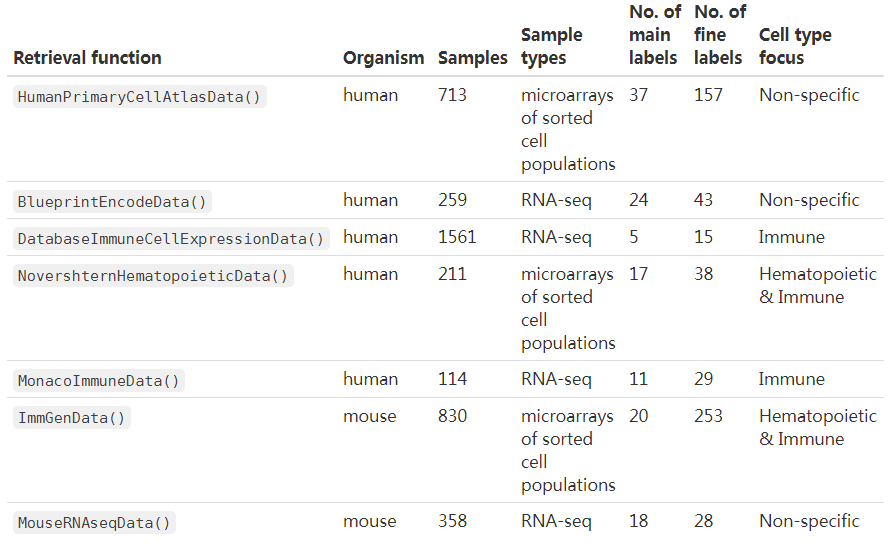
一共有7个参考数据集,其中5个人相关的(3个与免疫细胞相关),2个小鼠相关的
- Blueprint (Martens and Stunnenberg 2013) and Encode (The ENCODE Project Consortium 2012),
- the Human Primary Cell Atlas (Mabbott et al. 2013),
- the murine ImmGen (Heng et al. 2008), and
- a collection of mouse data sets downloaded from GEO (Benayoun et al. 2019).
免疫相关
- The Database for Immune Cell Expression(/eQTLs/Epigenomics) (Schmiedel et al. 2018),
- Novershtern Hematopoietic Cell Data - GSE24759 - formerly known as Differentiation Map (Novershtern et al. 2011), and
- Monaco Immune Cell Data - GSE107011 (Monaco et al. 2019).
关于相关数据集的下载可参考:
使用介绍
library(SingleR)# ###下载参考数据库# cg=BlueprintEncodeData()# cg=DatabaseImmuneCellExpressionData()# cg=NovershternHematopoieticData()# cg=MonacoImmuneData()# cg=ImmGenData()# cg=MouseRNAseqData()# cg=HumanPrimaryCellAtlasData()##加载参考数据集 人的参考数据hpca.se <- HumanPrimaryCellAtlasData()hpca.se##class: SummarizedExperiment##dim: 19363 713##metadata(0):##assays(1): logcounts##rownames(19363): A1BG A1BG-AS1 ... ZZEF1 ZZZ3##rowData names(0):##colnames(713): GSM112490 GSM112491 ... GSM92233 GSM92234##colData names(2): label.main label.fine###加载测试测试数据集library(scRNAseq)hESCs <- LaMannoBrainData('human-es')hESCs <- hESCs[,1:100]###利用前100数据进行测试
SingleR进行注释
##SingleR() expects log-counts, but the function will also happily take raw counts for the test dataset. The reference, however, must have log-values.library(scater)hESCs <- logNormCounts(hESCs)###使用HumanPrimaryCellAtlasData参考基因集进行注释pred.hesc <- SingleR(test = hESCs, ref = hpca.se, labels = hpca.se$label.main)pred.hesc
scores first.labels<matrix> <character>1772122_301_C02 0.118426779945786:0.179699807625087:0.157326274226517:... Neuroepithelial_cell1772122_180_E05 0.129708246318855:0.236277439793527:0.202370888668263:... Neuroepithelial_cell1772122_300_H02 0.158201338525345:0.250060222727419:0.211831550178353:... Neuroepithelial_cell1772122_180_B09 0.158778546217777:0.27716592787528:0.222681369744636:... Neuroepithelial_cell1772122_180_G04 0.138505219642345:0.236658649096383:0.19092437361406:... Neuroepithelial_cell... ... ...1772122_299_E07 0.145931041885859:0.241153701803065:0.217382763112476:... Neuroepithelial_cell1772122_180_D02 0.122983434596168:0.239181076829949:0.181221997276501:... Neuroepithelial_cell1772122_300_D09 0.129757310468164:0.233775092572195:0.196637664917917:... Neuroepithelial_cell1772122_298_F09 0.143118885460347:0.262267367714562:0.214329641867196:... Neuroepithelial_cell1772122_302_A11 0.0912854247387272:0.185945405472165:0.139232371863794:... Neuroepithelial_celltuning.scores labels pruned.labels<DataFrame> <character> <character>1772122_301_C02 0.18244020296249:0.0991115652997192 Neuroepithelial_cell Neuroepithelial_cell1772122_180_E05 0.137548373236792:0.0647133734667384 Neurons Neurons1772122_300_H02 0.275798157639906:0.136969040146444 Neuroepithelial_cell Neuroepithelial_cell1772122_180_B09 0.0851622797320583:0.0819878452425098 Neuroepithelial_cell Neuroepithelial_cell1772122_180_G04 0.198841544187094:0.101662168246495 Neuroepithelial_cell Neuroepithelial_cell... ... ... ...1772122_299_E07 0.176002520599547:0.0922503823656398 Neuroepithelial_cell Neuroepithelial_cell1772122_180_D02 0.196760862365318:0.112480486219438 Neuroepithelial_cell Neuroepithelial_cell1772122_300_D09 0.0816424287822026:0.0221368018363302 Neuroepithelial_cell Neuroepithelial_cell1772122_298_F09 0.187249853552379:0.0671892835266423 Neuroepithelial_cell Neuroepithelial_cell1772122_302_A11 0.156079956344163:0.105132159755961 Astrocyte Astrocyte
Labels are shown before fine-tuning (first.labels), after fine-tuning (labels) and after pruning (pruned.labels), along with the associated scores
table(pred.hesc$labels)Astrocyte Neuroepithelial_cell Neurons14 81 5
利用已标注的数据集对未标记的数据进行标注
The aim is to use one pre-labelled dataset to annotate the other unlabelled dataset.
library(scRNAseq)sceM <- MuraroPancreasData()# One should normally do cell-based quality control at this point, but for# brevity's sake, we will just remove the unlabelled libraries here.sceM <- sceM[,!is.na(sceM$label)]sceM <- logNormCounts(sceM)sceG <- GrunPancreasData()sceG <- sceG[,colSums(counts(sceG)) > 0] # Remove libraries with no counts.sceG <- logNormCounts(sceG)sceG <- sceG[,1:100]
对于单细胞数据而言,使用Wilcoxon 两两比较标记来识别标签。与默认的标记检测算法相比,这种方法速度较慢,但更适合单细胞数据(对于中值经常为零的低覆盖率数据,默认的标记检测算法可能失败)。
pred.grun <- SingleR(test=sceG, ref=sceM, labels=sceM$label, de.method="wilcox")
注释结果诊断
Based on the scores within cells
plotScoreHeatmap()displays the scores for all cells across all reference labels, which allows users to inspect the confidence of the predicted labels across the dataset.
plotScoreHeatmap(pred.grun)
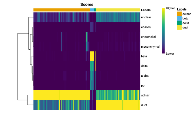
For this plot, the key point is to examine the spread of scores within each cell. Ideally, each cell (i.e., column of the heatmap) should have one score that is obviously larger than the rest, indicating that it is unambiguously assigned to a single label. A spread of similar scores for a given cell indicates that the assignment is uncertain, though this may be acceptable if the uncertainty is distributed across similar cell types that cannot be easily resolved.
查看每个cell中的值是否比其他值要高
plotScoreHeatmap(pred.grun,annotation_col=as.data.frame(colData(sceG)[,"donor",drop=FALSE]))
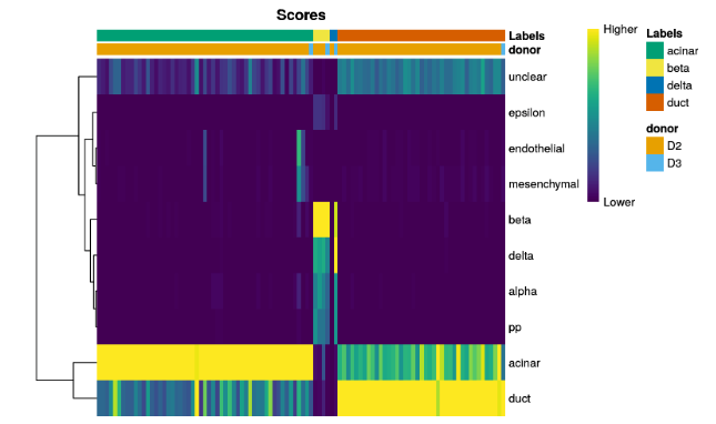
We can also display other metadata information for each cell by setting
clusters=orannotation_col=. This is occasionally useful for examining potential batch effects, differences in cell type composition between conditions, relationship to clusters from an unsupervised analysis, etc.
可以通过参数设置,查看数据来源和分组等相关信息。
Based on the deltas across cells
The
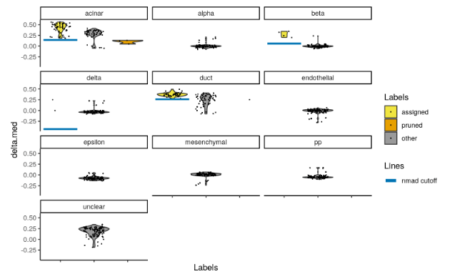
pruneScores()function will remove potentially poor-quality or ambiguous assignments. In particular, ambiguous assignments are identified based on the per-cell “delta”, i.e., the difference between the score for the assigned label and the median across all labels for each cell. Low deltas indicate that the assignment is uncertain, which is especially relevant if the cell’s true label does not exist in the reference. The exact threshold used for pruning is identified using an outlier-based approach that accounts for differences in the scale of the correlations in various contexts.
to.remove <- pruneScores(pred.grun)
By default,
SingleR()will report pruned labels in thepruned.labelsfield where low-quality assignments are replaced withNA. However, the default pruning thresholds may not be appropriate for every dataset - see?pruneScoresfor a more detailed discussion. We provide theplotScoreDistribution()to help in determining whether the thresholds are appropriate by using information across cells with the same label. This displays the per-label distribution of the deltas across cells, from whichpruneScores()defines an appropriate threshold as 3 median absolute deviations (MADs) below the median.
plotScoreDistribution(pred.grun, show = "delta.med", ncol = 3, show.nmads = 3)
If some tuning parameters must be adjusted, we can simply call
pruneScores()directly with adjusted parameters. Here, we set labels toNAif they are to be discarded, which is also howSingleR()marks such labels inpruned.labels.
new.pruned <- pred.grun$labelsnew.pruned[pruneScores(pred.grun, nmads=5)] <- NA
Based on marker gene expression
根据marker基因的表达情况,去识别注释效果
Another simple yet effective diagnostic is to examine the expression of the marker genes for each label in the test dataset. We extract the identity of the markers from the metadata of the
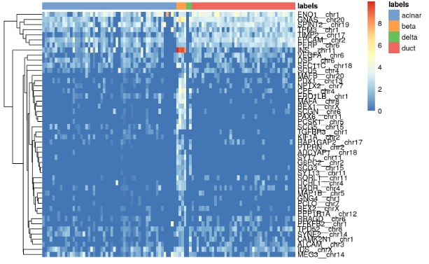
SingleR()results and use them in theplotHeatmap()function from scater, as shown below for beta cell markers. If a cell in the test dataset is confidently assigned to a particular label, we would expect it to have strong expression of that label’s markers. At the very least, it should exhibit upregulation of those markers relative to cells assigned to other labels.
all.markers <- metadata(pred.grun)$de.genessceG$labels <- pred.grun$labels# Beta cell-related markersplotHeatmap(sceG, order_columns_by="labels",features=unique(unlist(all.markers$beta)))
for (lab in unique(pred.grun$labels)) {plotHeatmap(sceG, order_columns_by=list(I(pred.grun$labels)),features=unique(unlist(all.markers[[lab]])))}
使用多个参考集进行注释
###使用多个参考数据集bp.se <- BlueprintEncodeData()pred.combined <- SingleR(test = hESCs,ref = list(BP=bp.se, HPCA=hpca.se),labels = list(bp.se$label.main, hpca.se$label.main))
使用
library(Seurat)sce <- readRDS("E:/single_seruat.Rds")sce_for_SingleR <- GetAssayData(sce, slot="data")mouseRNA <- MouseRNAseqData()pred.combined <- SingleR(test = sce_for_SingleR,ref = mouseRNA,labels = mouseRNA$label.main)sce[["SingleR.labels"]] <- pred.combined$labels

若有收获,就点个赞吧
0 人点赞
