参考资料:
Analysis, visualization, and integration of spatial datasets with Seurat
Seurat 新版教程:分析空间转录组数据
空间转录组流程
这篇笔记是参考以上的资料进行的学习记录
对于10X空间转录组数据而言,可以使用官方软件space ranger对原始数据进行处理。
主要的三个功能:
spaceranger mkfastq ##将bcl数据转换成fastq数据spaceranger count ##将fastq数据转换成空间特征矩阵spaceranger aggr ##可以将同分组,同流程的样本进行合并
处理流程大致如下: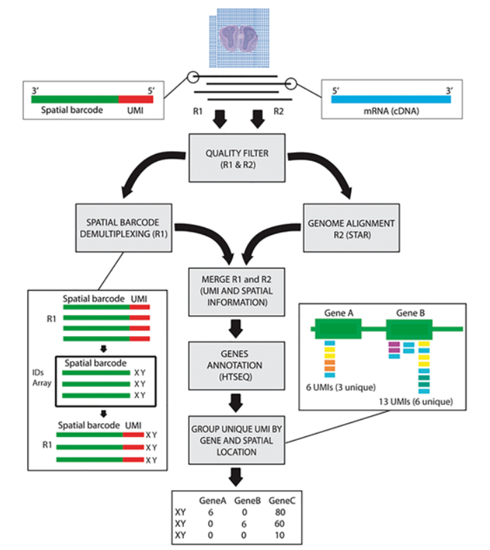
结果文件:
├── analysis|---├── clustering│---├── diffexp│---├── pca│---├── tsne│---└── umap├── cloupe.cloupe├── filtered_feature_bc_matrix ##需要的表达矩阵结果│---├── barcodes.tsv.gz│---├── features.tsv.gz│---└── matrix.mtx.gz├── filtered_feature_bc_matrix.h5 ##需要的表达矩阵结果├── metrics_summary.csv├── molecule_info.h5├── possorted_genome_bam.bam├── possorted_genome_bam.bam.bai├── raw_feature_bc_matrix│---├── barcodes.tsv.gz│---├── features.tsv.gz│---└── matrix.mtx.gz├── raw_feature_bc_matrix.h5├── spatial # 空间信息全在这 :这些文件是用户提供的原始全分辨率brightfield图像的下采样版本。下采样是通过box滤波实现的,它对全分辨率图像中像素块的RGB值进行平均,得到下采样图像中一个像素点的RGB值。│---├── aligned_fiducials.jpg 这个图像的尺寸是tissue_hires_image.png。由基准对齐算法发现的基准点用红色高亮显示。此文件对于验证基准对齐是否成功非常有用。│---├── detected_tissue_image.jpg│---├── scalefactors_json.json│---├── tissue_hires_image.png 图像的最大尺寸为2,000像素│---├── tissue_lowres_image.png 图像的最大尺寸为600像素。│---└── tissue_positions_list.csv└── web_summary.html
一般需要的是 filtered_feature_bc_matrix/filtered_feature_bc_matrix.h5数据,和对应的空间信息。
接下来利用Seurat流程进行分析。
数据读取
将h5数据和spatial数据放在同一文件夹下,利用Seurat包中的Load10X_Spatial函数进行读取。
?Load10X_SpatialLoad10X_Spatial(data.dir,filename = "filtered_feature_bc_matrix.h5",assay = "Spatial",slice = "slice1",filter.matrix = TRUE,to.upper = FALSE,...)data.dir: Directory containing the matrix.mtx, genes.tsv (or features.tsv), and barcodes.tsv files provided by 10X. A vector or named vector can be given in order to load several data directories. If a named vector is given, the cell barcode names will be prefixed with the name.filename: Name of H5 file containing the feature barcode matrix, ps:默认读取的是"filtered_feature_bc_matrix.h5"文件assay : Name of the initial assayslice : Name for the stored image of the tissue slicefilter.matrix : Only keep spots that have been determined to be over tissueto.upper : Converts all feature names to upper case. Can be useful when analyses require comparisons between human and mouse gene names for example.brain<-Seurat::Load10X_Spatial("data/V1_Mouse_Brain_Sagittal_Anterio/")
The visium data from 10x consists of the following data types:
- A spot by gene expression matrix
- An image of the tissue slice (obtained from H&E staining during data acquisition)
- Scaling factors that relate the original high resolution image to the lower resolution image used here for visualization.
In the Seurat object, the spot by gene expression matrix is similar to a typical “RNA” Assay but contains spot level, not single-cell level data. The image itself is stored in a new images slot in the Seurat object. The images slot also stores the information necessary to associate spots with their physical position on the tissue image.
数据预处理
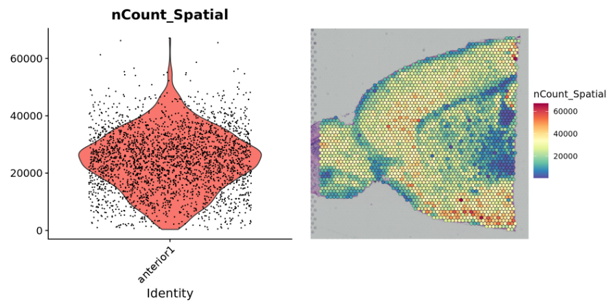
###数据在切片上的整体基因表达情况plot1 <- VlnPlot(brain, features = "nCount_Spatial", pt.size = 0.1) + NoLegend()plot2 <- SpatialFeaturePlot(brain, features = "nCount_Spatial") + theme(legend.position = "right")wrap_plots(plot1, plot2)
需要对数据进行标准化处理,从而减少测序深度带来的影响
同时,因为组织中细胞的密度差异原因,使得数据存在异质性,所以需要进行有效的Normalization,但是因为组织特异性的原因,常规的标准化方法(LogNormalize)不适用。
Seurat推荐使用SCTransform()进行标准化处理
###对数据进行标准化处理brain <- SCTransform(brain, assay = "Spatial", verbose = FALSE)
基因表达的可视化
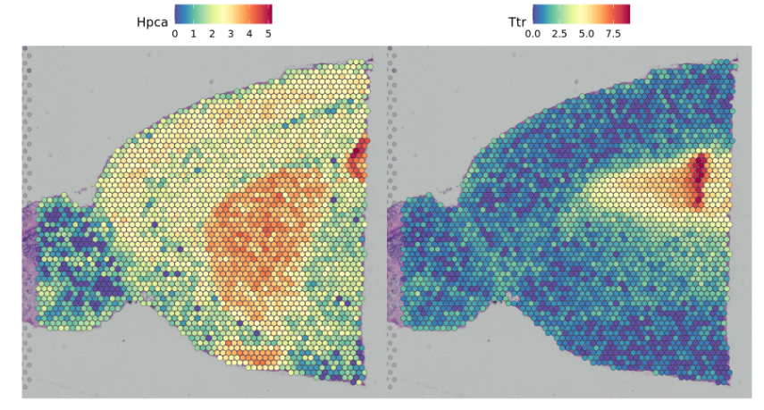
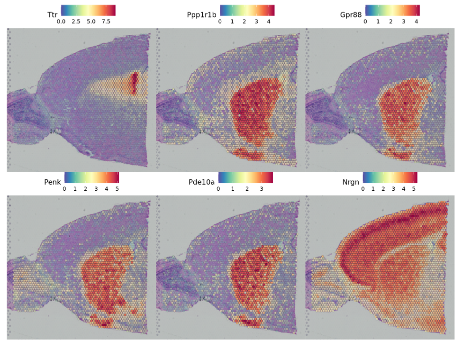
可以使用Seurat中的SpatialFeaturePlot函数来查看组织上的相关基因的表达情况
SpatialFeaturePlot(brain, features = c("Hpca", "Ttr"))
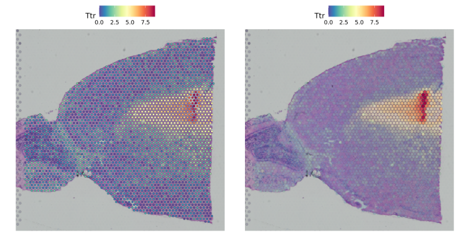
##相关参数设置pt.size.factor- This will scale the size of the spots. Default is 1.6alpha - minimum and maximum transparency. Default is c(1, 1).Try setting to alpha c(0.1, 1), to downweight the transparency of points with lower expression#相关参数修改p1 <- SpatialFeaturePlot(brain, features = "Ttr", pt.size.factor = 1)p2 <- SpatialFeaturePlot(brain, features = "Ttr", alpha = c(0.1, 1))p1 + p2
降维、聚类、可视化
使用与scRNA-seq分析相同的工作流程,对空间转录组数据进行聚类。使用 graph-based clustering approach方法进行聚类。
brain <- RunPCA(brain, assay = "SCT", verbose = FALSE)brain <- FindNeighbors(brain, reduction = "pca", dims = 1:30)brain <- FindClusters(brain, verbose = FALSE)brain <- RunUMAP(brain, reduction = "pca", dims = 1:30)
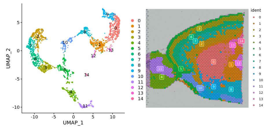
使用DimPlot函数或SpatialDimPlot函数对cluster进行展示和查看。
####可视化查看p1 <- DimPlot(brain, reduction = "umap", label = TRUE)p2 <- SpatialDimPlot(brain, label = TRUE, label.size = 3)p1 + p2
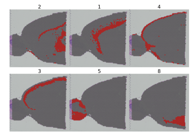
You can also use the cells.highlight parameter to demarcate particular cells of interest on a SpatialDimPlot
SpatialDimPlot函数中的cells.highlight参数可以查看指定的cluster。
##查看特定类的情况SpatialDimPlot(brain, cells.highlight = CellsByIdentities(object = brain, idents = c(2, 1, 4, 3, 5, 8)), facet.highlight = TRUE, ncol = 3)
交互式的可视化
Both SpatialDimPlot and SpatialFeaturePlot now have an interactive parameter, that when set to TRUE, will open up the Rstudio viewer pane with an interactive Shiny plot.
##Interactive plottingSpatialDimPlot(brain, interactive = TRUE)
For SpatialFeaturePlot, setting interactive to TRUE brings up an interactive pane in which you can adjust the transparency of the spots, the point size, as well as the Assay and feature being plotted.
SpatialFeaturePlot(brain, features = "Ttr", interactive = TRUE)
The LinkedDimPlot function links the UMAP representation to the tissue image representation and allows for interactive selection.
LinkedDimPlot(brain)
识别空间变量的特性
- The first is to perform differential expression based on pre-annotated anatomical regions within the tissue, which may be determined either from unsupervised clustering or prior knowledge.This strategy works will in this case, as the clusters above exhibit clear spatial restriction.
第一种是基于组织内预先注释的解剖区域来进行差异表达,这可以通过无监督聚类或先验知识来确定。
##识别两个cluster中的差异基因de_markers <- FindMarkers(brain, ident.1 = 4, ident.2 = 6)SpatialFeaturePlot(object = brain, features = rownames(de_markers)[1:3], alpha = c(0.1, 1), ncol = 3)
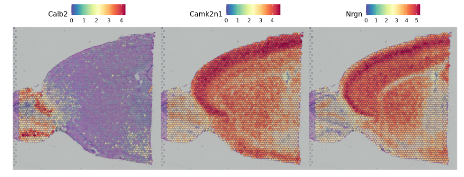
- An alternative approach, implemented in
FindSpatiallyVariables, is to search for features exhibiting spatial patterning in the absence of pre-annotation. The default method (method = 'markvariogram).
另一种方法是在没有预先注释的情况下,寻找显示空间模式的特征。利用FindSpatiallyVariables函数进行实现。
brain <- FindSpatiallyVariableFeatures(brain, assay = "SCT", features = VariableFeatures(brain)[1:1000], selection.method = "markvariogram")###查看显著的基因top.features <- head(SpatiallyVariableFeatures(brain, selection.method = "markvariogram"), 6)SpatialFeaturePlot(brain, features = top.features, ncol = 3, alpha = c(0.1, 1))
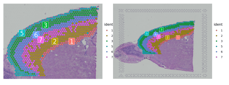
划分解剖区域
###Subset out anatomical regions 划分解剖区域cortex <- subset(brain, idents = c(1, 2, 3, 5, 6, 7))# now remove additional cells, use SpatialDimPlots to visualize what to remove# SpatialDimPlot(cortex,cells.highlight = WhichCells(cortex, expression = image_imagerow > 400 | image_imagecol < 150))cortex <- subset(cortex, anterior1_imagerow > 400 | anterior1_imagecol < 150, invert = TRUE)cortex <- subset(cortex, anterior1_imagerow > 275 & anterior1_imagecol > 370, invert = TRUE)cortex <- subset(cortex, anterior1_imagerow > 250 & anterior1_imagecol > 440, invert = TRUE)###p1 <- SpatialDimPlot(cortex, crop = TRUE, label = TRUE)p2 <- SpatialDimPlot(cortex, crop = FALSE, label = TRUE, pt.size.factor = 1, label.size = 3)p1 + p2
与单细胞数据关联分析(空间细胞类型定义)
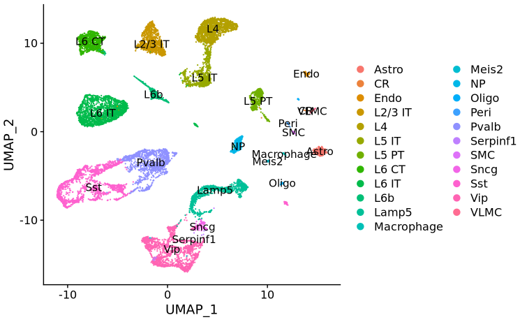
预处理scRNA-seq 参考数据集,然后执行标签传输。该过程为每个spot输出每个scRNA-seq派生类的概率分类。我们将这些预测添加到Seurat对象中作为新的试验。
allen_reference <- readRDS("~/Downloads/allen_cortex.rds")# note that setting ncells=3000 normalizes the full dataset but learns noise models on 3k cells# this speeds up SCTransform dramatically with no loss in performancelibrary(dplyr)allen_reference <- SCTransform(allen_reference, ncells = 3000, verbose = FALSE) %>% RunPCA(verbose = FALSE) %>% RunUMAP(dims = 1:30)# After subsetting, we renormalize cortexcortex <- SCTransform(cortex, assay = "Spatial", verbose = FALSE) %>% RunPCA(verbose = FALSE)# the annotation is stored in the 'subclass' column of object metadataDimPlot(allen_reference, group.by = "subclass", label = TRUE)
获得每个class的每个spot的预测分数
# get prediction scores for each spot for each classanchors <- FindTransferAnchors(reference = allen_reference, query = cortex, normalization.method = "SCT")predictions.assay <- TransferData(anchorset = anchors, refdata = allen_reference$subclass, prediction.assay = TRUE, weight.reduction = cortex[["pca"]])cortex[["predictions"]] <- predictions.assay
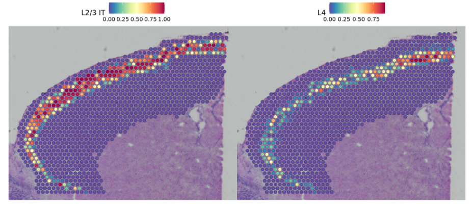
Here we can distinguish between distinct sequential layers of these neuronal subtypes
在这里,我们可以区分这些神经元亚型的不同顺序层
DefaultAssay(cortex) <- "predictions"SpatialFeaturePlot(cortex, features = c("L2/3 IT", "L4"), pt.size.factor = 1.6, ncol = 2, crop = TRUE)
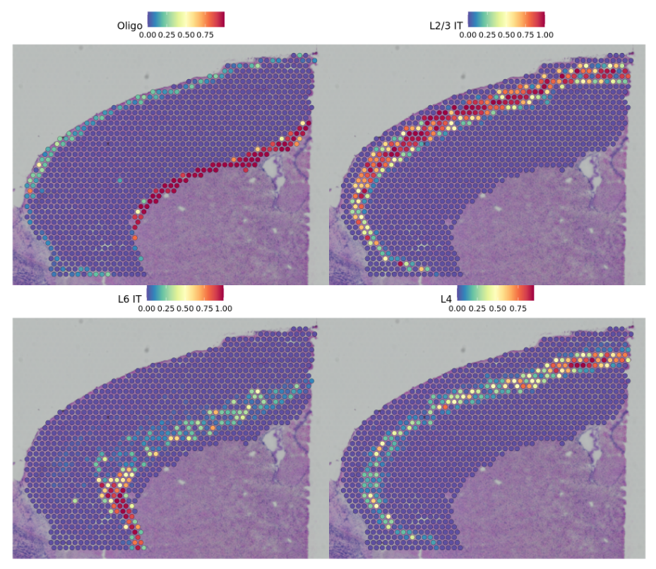
Based on these prediction scores, we can also predict cell types whose location is spatially restricted. 利用预测得分获得细胞类型
We use the same methods based on marked point processes to define spatially variable features, but use the cell type prediction scores as the “marks” rather than gene expression. 利用预测得分去定义空间变量特征
cortex <- FindSpatiallyVariableFeatures(cortex, assay = "predictions", selection.method = "markvariogram", features = rownames(cortex), r.metric = 5, slot = "data")top.clusters <- head(SpatiallyVariableFeatures(cortex), 4)SpatialPlot(object = cortex, features = top.clusters, ncol = 2)
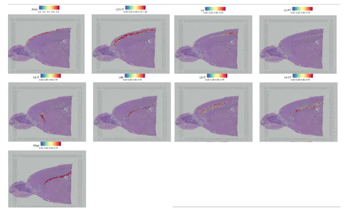
show that our integrative procedure
SpatialFeaturePlot(cortex, features = c("Astro", "L2/3 IT", "L4", "L5 PT", "L5 IT", "L6 CT", "L6 IT","L6b", "Oligo"), pt.size.factor = 1, ncol = 2, crop = FALSE, alpha = c(0.1, 1))
Working with multiple slices in Seurat
##Working with multiple slices in Seuratbrain2 <- LoadData("stxBrain", type = "posterior1")brain2 <- SCTransform(brain2, assay = "Spatial", verbose = FALSE)###merge函数合并数据brain.merge <- merge(brain, brain2)###聚类DefaultAssay(brain.merge) <- "SCT"VariableFeatures(brain.merge) <- c(VariableFeatures(brain), VariableFeatures(brain2))brain.merge <- RunPCA(brain.merge, verbose = FALSE)brain.merge <- FindNeighbors(brain.merge, dims = 1:30)brain.merge <- FindClusters(brain.merge, verbose = FALSE)brain.merge <- RunUMAP(brain.merge, dims = 1:30)##查看DimPlot(brain.merge, reduction = "umap", group.by = c("ident", "orig.ident"))SpatialDimPlot(brain.merge)SpatialFeaturePlot(brain.merge, features = c("Hpca", "Plp1"))

若有收获,就点个赞吧
0 人点赞
