2.1 导读
单细胞数据预处理准备完毕之后、需要以下步骤
- 数据标准化
- 查找高变基因
- PCA分析
- 去除批次效应 (可选)
-
2.2 数据处理
数据标准化
sc.pp.normalize_per_cell(adata_all, counts_per_cell_after=1e4)sc.pp.log1p(adata_all)
查找高变基因
sc.pp.highly_variable_genes(adata_all, n_top_genes =1500, batch_key='sample')sc.pl.highly_variable_genes(adata_all)
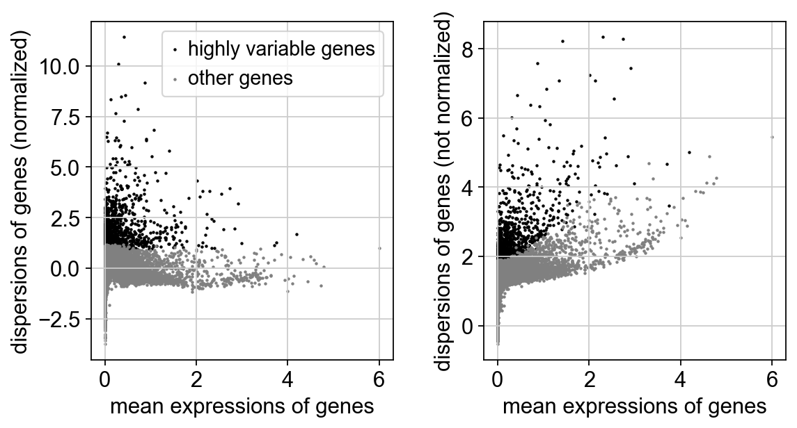
- 识别差异表达基因
- n_top_genes 参数设置 高变基因个数
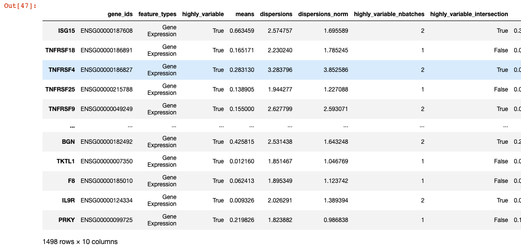
过滤高变基因中线粒体等
adata_all.var.highly_variable = adata_all.var.highly_variable & [ not x.startswith(('RPL', 'RPS', 'MT-', 'MRPS', 'MRPL')) for x in adata_all.var.index ]adata_all.var[adata_all.var['highly_variable']]
PCA 主成分分析
sc.pp.scale( adata_all, max_value=10)sc.tl.pca( adata_all, svd_solver='arpack', n_comps=20, use_highly_variable = True)sc.pl.pca(adata_all, color='GAB3') #绘图
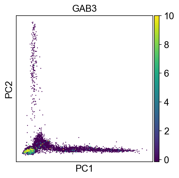
- 主成分分析是一种将数据降维的分析方法,是考察多个变量间相关性一种多元统计方法,研究如何通过少数几个主成分来揭示多个变量间的内部结构,即从原始变量中导出少数几个主成分,使它们尽可能多地保留原始变量的信息,且彼此间互不相关.通常数学上的处理就是将原来P个指标作线性组合,作为新的综合指标。
- 通过运行主成分分析 (PCA) 来降低数据的维数,可以对数据进行去噪并揭示不同分群的主因素。
去除批次效应
# 按照样本进行批次效应去除sc.external.pp.harmony_integrate(adata_all, 'sample',basis = 'X_pca',adjusted_basis= 'X_pca_harmony',)
计算细胞间的距离
sc.pp.neighbors(adata_all, n_pcs=20, use_rep= 'X_pca_harmony')
- 这里的参数就先按照默认值设定:
- 使用数据矩阵的 PCA去次批次效应之后 表示来计算细胞的邻域图。
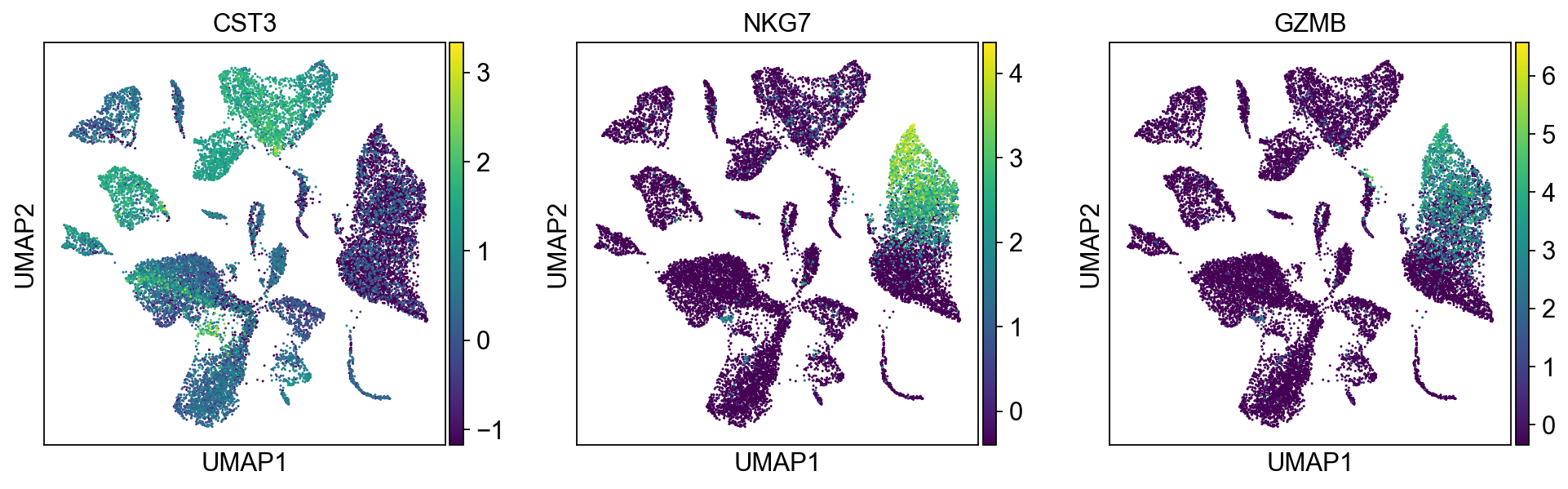
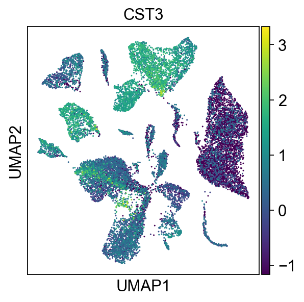
umap降维分析
sc.tl.umap(adata_all,)sc.pl.umap(adata_all, color=['CST3', 'NKG7',"GZMB"],)
# 按照样本查看sc.pl.umap(adata_all, color=['CST3'],groups="sample")
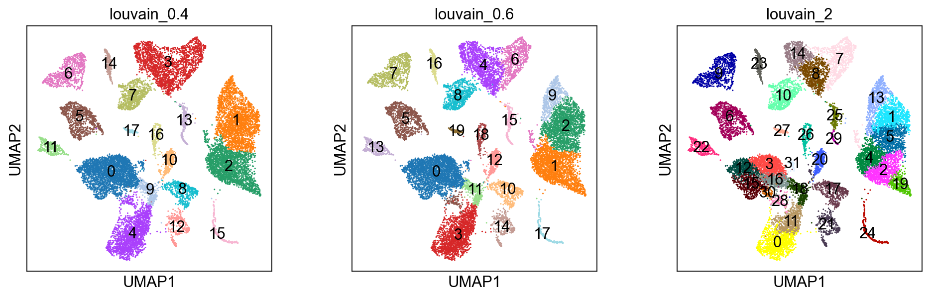
聚类分析
# 可以按照不同的resolution 进行聚类sc.tl.louvain(adata_all,resolution=0.4,key_added="louvain_0.4")sc.tl.louvain(adata_all,resolution=0.6,key_added="louvain_0.6")sc.tl.louvain(adata_all,resolution=2,key_added="louvain_2")sc.pl.umap(adata_all, color=['louvain_0.4','louvain_0.6','louvain_2'],legend_loc='on data')
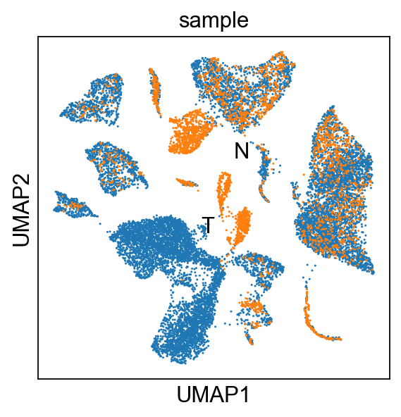
sc.pl.umap(adata_all, color="sample",legend_loc='on data')
2.3 基因数据
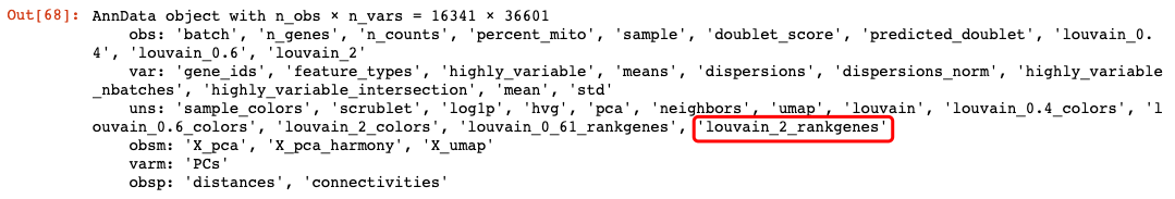
查找聚类Marker基因,以resolution= 2 为例。
sc.tl.rank_genes_groups(adata_all, 'louvain_2', method='wilcoxon',key_added='louvain_2_rankgenes')adata_all
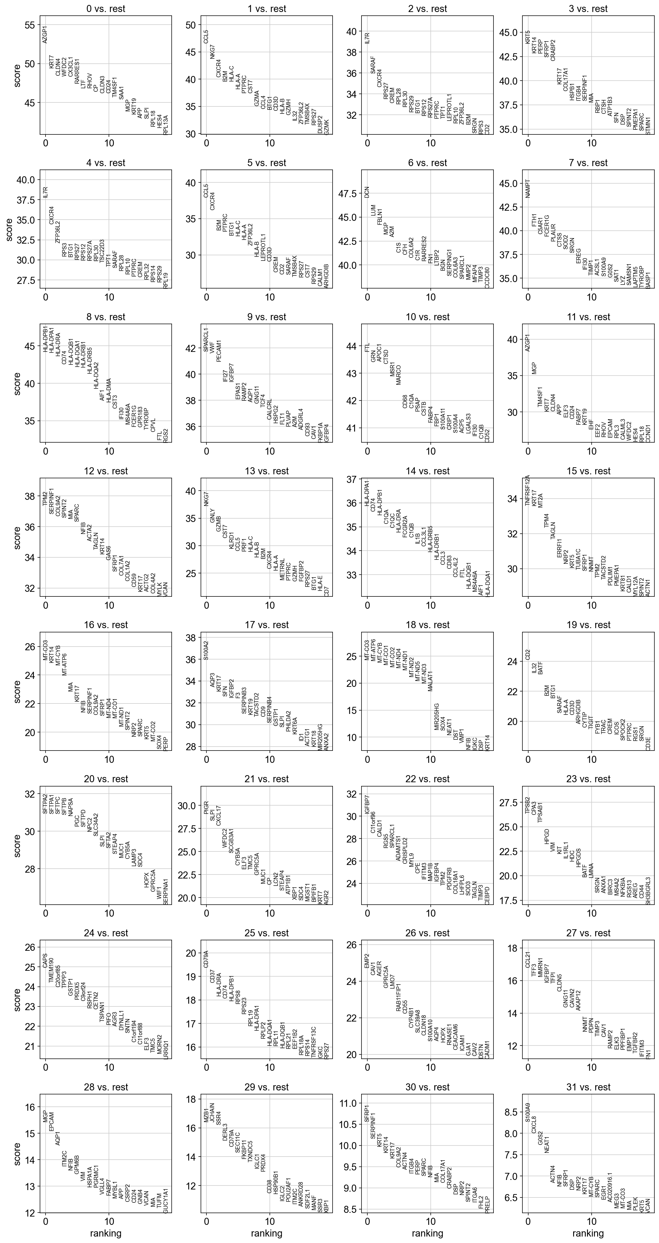
查看top20 Marker基因
sc.pl.rank_genes_groups(adata_all, n_genes=20, sharey=False,key='louvain_2_rankgenes')
提取Marker基因
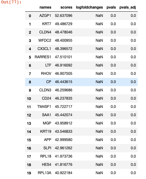
提取cluster 0 marker基因
df_markergene_0 = sc.get.rank_genes_groups_df(adata_all, group="0",key= "louvain_2_rankgenes")df_markergene_0[0:20]
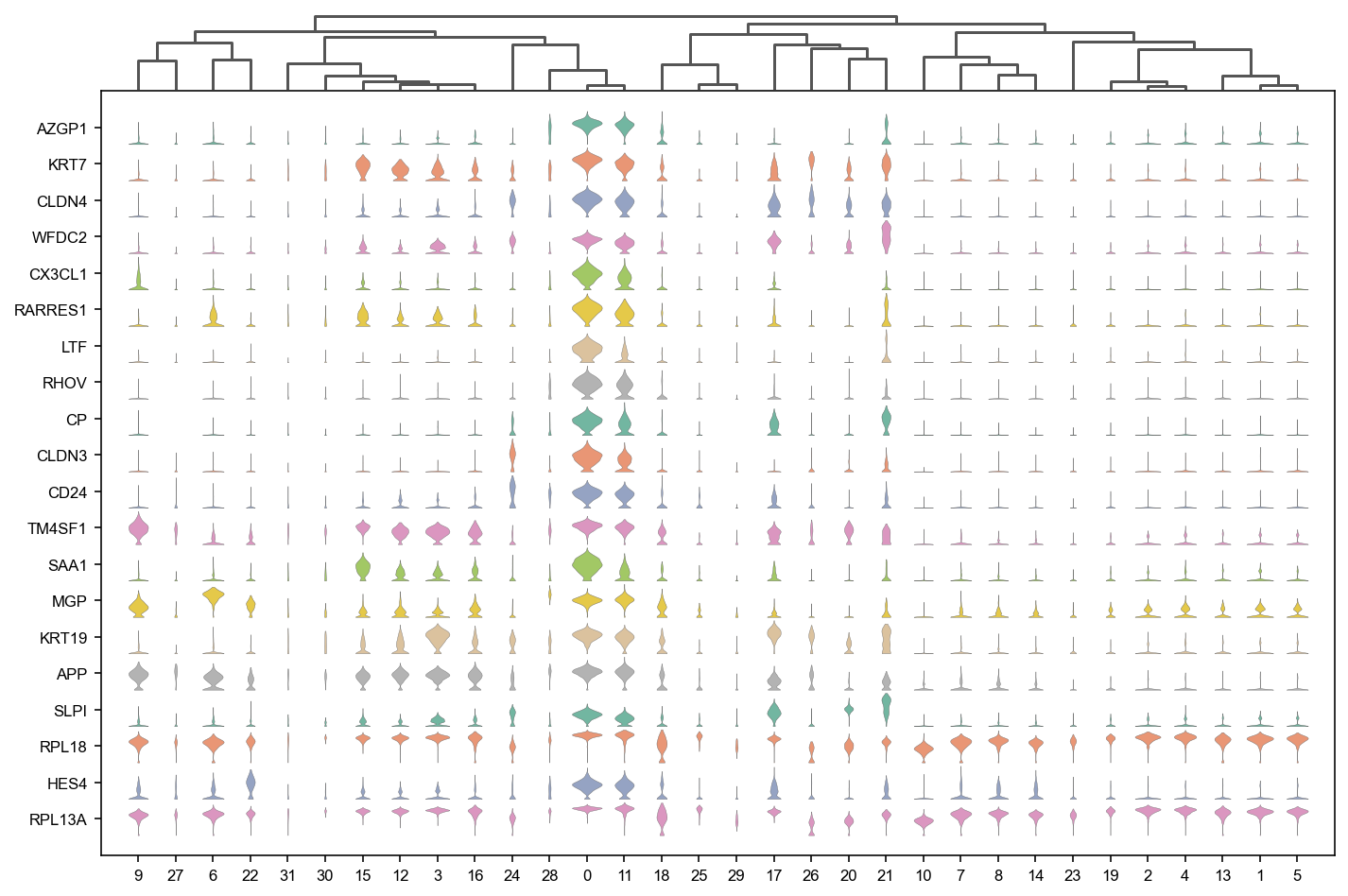
用cluster 0 marker基因画图 按照cluster聚类
sc.pl.stacked_violin(adata_all,list(df_markergene_0[0:20]['names']), groupby="louvain_2",use_raw=False, dendrogram=True, standard_scale ='var',row_palette = 'Set2',scale='count',swap_axes=True)
下一遍会具体讲述 数据画图技巧。
总结
到此 数据简单处理完毕


若有收获,就点个赞吧
0 人点赞
