实验要求：

以kNN和SVM算法为例，理解分类分析算法的基本原理及流程，理解kNN和SVM算法的区别。
利用kNN算法，以参数k=3编程对鸢尾花进行分类，建议使用sklearn中内置的已经预处理好的数据集。
输出训练好的模型在训练集与测试集上的分类准确度。
对测试集上数据预测的结果进行可视化输出，与真值进行对比。
使用SVM算法训练模型，计算训练好的模型在训练集与测试集上的分类准确度。
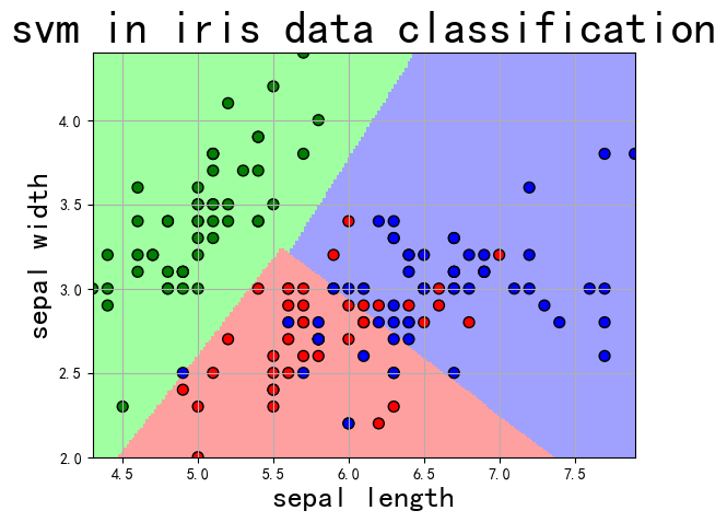
选择数据的其中两维，可视化输出SVM模型的分类边界。

注：

训练集与测试集均可通过原数据集抽样取得，可考虑使用train_test_split方法（在sklearn.model_selection中）。
kNN算法和SVM算法在sklearn中均有实现，不建议各位同学手动编写，否则工作量会过于庞大。若感兴趣，也欢迎在课后自行研究。
kNN算法及SVM算法都涉及到模型参数，同学们可以尝试不同的参数并观察准确率。
由于我们在二维平面上绘制SVM模型分类边界，视代码实现方式可能需要重新训练模型。

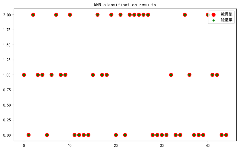
可视化输出示例：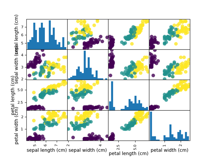

上机实现：

KNN实现：

导入需要的数据集和包

from sklearn.datasets import load_iris
from sklearn.model_selection import train_test_split
from sklearn.neighbors import KNeighborsClassifier
from sklearn.metrics import accuracy_score
import matplotlib.pyplot as plt
import seaborn as sns
import pandas as pd
plt.rcParams["font.sans-serif"] = ["SimHei"]

获取数据

load_iris()
iris = load_iris()
iris

{'data': array([[5.1, 3.5, 1.4, 0.2],
        [4.9, 3. , 1.4, 0.2],
        [4.7, 3.2, 1.3, 0.2],
        [4.6, 3.1, 1.5, 0.2],
        [5. , 3.6, 1.4, 0.2],
        [5.4, 3.9, 1.7, 0.4],
        [4.6, 3.4, 1.4, 0.3],
        [5. , 3.4, 1.5, 0.2],
        [4.4, 2.9, 1.4, 0.2],
        [4.9, 3.1, 1.5, 0.1],
        [5.4, 3.7, 1.5, 0.2],
        [4.8, 3.4, 1.6, 0.2],
        [4.8, 3. , 1.4, 0.1],
        [4.3, 3. , 1.1, 0.1],
        [5.8, 4. , 1.2, 0.2],
        [5.7, 4.4, 1.5, 0.4],
        [5.4, 3.9, 1.3, 0.4],
        [5.1, 3.5, 1.4, 0.3],
        [5.7, 3.8, 1.7, 0.3],
        [5.1, 3.8, 1.5, 0.3],
        [5.4, 3.4, 1.7, 0.2],
        [5.1, 3.7, 1.5, 0.4],
        [4.6, 3.6, 1. , 0.2],
        [5.1, 3.3, 1.7, 0.5],
        [4.8, 3.4, 1.9, 0.2],
        [5. , 3. , 1.6, 0.2],
        [5. , 3.4, 1.6, 0.4],
        [5.2, 3.5, 1.5, 0.2],
        [5.2, 3.4, 1.4, 0.2],
        [4.7, 3.2, 1.6, 0.2],
        [4.8, 3.1, 1.6, 0.2],
        [5.4, 3.4, 1.5, 0.4],
        [5.2, 4.1, 1.5, 0.1],
        [5.5, 4.2, 1.4, 0.2],
        [4.9, 3.1, 1.5, 0.2],
        [5. , 3.2, 1.2, 0.2],
        [5.5, 3.5, 1.3, 0.2],
        [4.9, 3.6, 1.4, 0.1],
        [4.4, 3. , 1.3, 0.2],
        [5.1, 3.4, 1.5, 0.2],
        [5. , 3.5, 1.3, 0.3],
        [4.5, 2.3, 1.3, 0.3],
        [4.4, 3.2, 1.3, 0.2],
        [5. , 3.5, 1.6, 0.6],
        [5.1, 3.8, 1.9, 0.4],
        [4.8, 3. , 1.4, 0.3],
        [5.1, 3.8, 1.6, 0.2],
        [4.6, 3.2, 1.4, 0.2],
        [5.3, 3.7, 1.5, 0.2],
        [5. , 3.3, 1.4, 0.2],
        [7. , 3.2, 4.7, 1.4],
        [6.4, 3.2, 4.5, 1.5],
        [6.9, 3.1, 4.9, 1.5],
        [5.5, 2.3, 4. , 1.3],
        [6.5, 2.8, 4.6, 1.5],
        [5.7, 2.8, 4.5, 1.3],
        [6.3, 3.3, 4.7, 1.6],
        [4.9, 2.4, 3.3, 1. ],
        [6.6, 2.9, 4.6, 1.3],
        [5.2, 2.7, 3.9, 1.4],
        [5. , 2. , 3.5, 1. ],
        [5.9, 3. , 4.2, 1.5],
        [6. , 2.2, 4. , 1. ],
        [6.1, 2.9, 4.7, 1.4],
        [5.6, 2.9, 3.6, 1.3],
        [6.7, 3.1, 4.4, 1.4],
        [5.6, 3. , 4.5, 1.5],
        [5.8, 2.7, 4.1, 1. ],
        [6.2, 2.2, 4.5, 1.5],
        [5.6, 2.5, 3.9, 1.1],
        [5.9, 3.2, 4.8, 1.8],
        [6.1, 2.8, 4. , 1.3],
        [6.3, 2.5, 4.9, 1.5],
        [6.1, 2.8, 4.7, 1.2],
        [6.4, 2.9, 4.3, 1.3],
        [6.6, 3. , 4.4, 1.4],
        [6.8, 2.8, 4.8, 1.4],
        [6.7, 3. , 5. , 1.7],
        [6. , 2.9, 4.5, 1.5],
        [5.7, 2.6, 3.5, 1. ],
        [5.5, 2.4, 3.8, 1.1],
        [5.5, 2.4, 3.7, 1. ],
        [5.8, 2.7, 3.9, 1.2],
        [6. , 2.7, 5.1, 1.6],
        [5.4, 3. , 4.5, 1.5],
        [6. , 3.4, 4.5, 1.6],
        [6.7, 3.1, 4.7, 1.5],
        [6.3, 2.3, 4.4, 1.3],
        [5.6, 3. , 4.1, 1.3],
        [5.5, 2.5, 4. , 1.3],
        [5.5, 2.6, 4.4, 1.2],
        [6.1, 3. , 4.6, 1.4],
        [5.8, 2.6, 4. , 1.2],
        [5. , 2.3, 3.3, 1. ],
        [5.6, 2.7, 4.2, 1.3],
        [5.7, 3. , 4.2, 1.2],
        [5.7, 2.9, 4.2, 1.3],
        [6.2, 2.9, 4.3, 1.3],
        [5.1, 2.5, 3. , 1.1],
        [5.7, 2.8, 4.1, 1.3],
        [6.3, 3.3, 6. , 2.5],
        [5.8, 2.7, 5.1, 1.9],
        [7.1, 3. , 5.9, 2.1],
        [6.3, 2.9, 5.6, 1.8],
        [6.5, 3. , 5.8, 2.2],
        [7.6, 3. , 6.6, 2.1],
        [4.9, 2.5, 4.5, 1.7],
        [7.3, 2.9, 6.3, 1.8],
        [6.7, 2.5, 5.8, 1.8],
        [7.2, 3.6, 6.1, 2.5],
        [6.5, 3.2, 5.1, 2. ],
        [6.4, 2.7, 5.3, 1.9],
        [6.8, 3. , 5.5, 2.1],
        [5.7, 2.5, 5. , 2. ],
        [5.8, 2.8, 5.1, 2.4],
        [6.4, 3.2, 5.3, 2.3],
        [6.5, 3. , 5.5, 1.8],
        [7.7, 3.8, 6.7, 2.2],
        [7.7, 2.6, 6.9, 2.3],
        [6. , 2.2, 5. , 1.5],
        [6.9, 3.2, 5.7, 2.3],
        [5.6, 2.8, 4.9, 2. ],
        [7.7, 2.8, 6.7, 2. ],
        [6.3, 2.7, 4.9, 1.8],
        [6.7, 3.3, 5.7, 2.1],
        [7.2, 3.2, 6. , 1.8],
        [6.2, 2.8, 4.8, 1.8],
        [6.1, 3. , 4.9, 1.8],
        [6.4, 2.8, 5.6, 2.1],
        [7.2, 3. , 5.8, 1.6],
        [7.4, 2.8, 6.1, 1.9],
        [7.9, 3.8, 6.4, 2. ],
        [6.4, 2.8, 5.6, 2.2],
        [6.3, 2.8, 5.1, 1.5],
        [6.1, 2.6, 5.6, 1.4],
        [7.7, 3. , 6.1, 2.3],
        [6.3, 3.4, 5.6, 2.4],
        [6.4, 3.1, 5.5, 1.8],
        [6. , 3. , 4.8, 1.8],
        [6.9, 3.1, 5.4, 2.1],
        [6.7, 3.1, 5.6, 2.4],
        [6.9, 3.1, 5.1, 2.3],
        [5.8, 2.7, 5.1, 1.9],
        [6.8, 3.2, 5.9, 2.3],
        [6.7, 3.3, 5.7, 2.5],
        [6.7, 3. , 5.2, 2.3],
        [6.3, 2.5, 5. , 1.9],
        [6.5, 3. , 5.2, 2. ],
        [6.2, 3.4, 5.4, 2.3],
        [5.9, 3. , 5.1, 1.8]]),
 'target': array([0, 0, 0, 0, 0, 0, 0, 0, 0, 0, 0, 0, 0, 0, 0, 0, 0, 0, 0, 0, 0, 0,
        0, 0, 0, 0, 0, 0, 0, 0, 0, 0, 0, 0, 0, 0, 0, 0, 0, 0, 0, 0, 0, 0,
        0, 0, 0, 0, 0, 0, 1, 1, 1, 1, 1, 1, 1, 1, 1, 1, 1, 1, 1, 1, 1, 1,
        1, 1, 1, 1, 1, 1, 1, 1, 1, 1, 1, 1, 1, 1, 1, 1, 1, 1, 1, 1, 1, 1,
        1, 1, 1, 1, 1, 1, 1, 1, 1, 1, 1, 1, 2, 2, 2, 2, 2, 2, 2, 2, 2, 2,
        2, 2, 2, 2, 2, 2, 2, 2, 2, 2, 2, 2, 2, 2, 2, 2, 2, 2, 2, 2, 2, 2,
        2, 2, 2, 2, 2, 2, 2, 2, 2, 2, 2, 2, 2, 2, 2, 2, 2, 2]),
 'frame': None,
 'target_names': array(['setosa', 'versicolor', 'virginica'], dtype='<U10'),
 'DESCR': '.. _iris_dataset:\n\nIris plants dataset\n--------------------\n\n**Data Set Characteristics:**\n\n    :Number of Instances: 150 (50 in each of three classes)\n    :Number of Attributes: 4 numeric, predictive attributes and the class\n    :Attribute Information:\n        - sepal length in cm\n        - sepal width in cm\n        - petal length in cm\n        - petal width in cm\n        - class:\n                - Iris-Setosa\n                - Iris-Versicolour\n                - Iris-Virginica\n                \n    :Summary Statistics:\n\n    ============== ==== ==== ======= ===== ====================\n                    Min  Max   Mean    SD   Class Correlation\n    ============== ==== ==== ======= ===== ====================\n    sepal length:   4.3  7.9   5.84   0.83    0.7826\n    sepal width:    2.0  4.4   3.05   0.43   -0.4194\n    petal length:   1.0  6.9   3.76   1.76    0.9490  (high!)\n    petal width:    0.1  2.5   1.20   0.76    0.9565  (high!)\n    ============== ==== ==== ======= ===== ====================\n\n    :Missing Attribute Values: None\n    :Class Distribution: 33.3% for each of 3 classes.\n    :Creator: R.A. Fisher\n    :Donor: Michael Marshall (MARSHALL%PLU@io.arc.nasa.gov)\n    :Date: July, 1988\n\nThe famous Iris database, first used by Sir R.A. Fisher. The dataset is taken\nfrom Fisher\'s paper. Note that it\'s the same as in R, but not as in the UCI\nMachine Learning Repository, which has two wrong data points.\n\nThis is perhaps the best known database to be found in the\npattern recognition literature.  Fisher\'s paper is a classic in the field and\nis referenced frequently to this day.  (See Duda & Hart, for example.)  The\ndata set contains 3 classes of 50 instances each, where each class refers to a\ntype of iris plant.  One class is linearly separable from the other 2; the\nlatter are NOT linearly separable from each other.\n\n.. topic:: References\n\n   - Fisher, R.A. "The use of multiple measurements in taxonomic problems"\n     Annual Eugenics, 7, Part II, 179-188 (1936); also in "Contributions to\n     Mathematical Statistics" (John Wiley, NY, 1950).\n   - Duda, R.O., & Hart, P.E. (1973) Pattern Classification and Scene Analysis.\n     (Q327.D83) John Wiley & Sons.  ISBN 0-471-22361-1.  See page 218.\n   - Dasarathy, B.V. (1980) "Nosing Around the Neighborhood: A New System\n     Structure and Classification Rule for Recognition in Partially Exposed\n     Environments".  IEEE Transactions on Pattern Analysis and Machine\n     Intelligence, Vol. PAMI-2, No. 1, 67-71.\n   - Gates, G.W. (1972) "The Reduced Nearest Neighbor Rule".  IEEE Transactions\n     on Information Theory, May 1972, 431-433.\n   - See also: 1988 MLC Proceedings, 54-64.  Cheeseman et al"s AUTOCLASS II\n     conceptual clustering system finds 3 classes in the data.\n   - Many, many more ...',
 'feature_names': ['sepal length (cm)',
  'sepal width (cm)',
  'petal length (cm)',
  'petal width (cm)'],
 'filename': 'iris.csv',
 'data_module': 'sklearn.datasets.data'}

数据集的说明

#特征
fea = iris.data
#目标
lab = iris.target#【重要】
#目标的名称
tar_nm = iris.target_names
#特征列名称
fea_nm = iris.feature_names
pd.DataFrame(data = fea, columns = fea_nm)
pd.DataFrame(tar_nm[lab],columns=['labels'])
#制作dataframe
fea_df = pd.DataFrame(data=fea,columns=fea_nm)
lab_df = pd.DataFrame(tar_nm[lab],columns=['labels'])#【重要】
df =pd.concat([fea_df,lab_df],axis=1,join='inner')
df.describe()

	sepal length (cm)	sepal width (cm)	petal length (cm)	petal width (cm)
count	150.000000	150.000000	150.000000	150.000000
mean	5.843333	3.057333	3.758000	1.199333
std	0.828066	0.435866	1.765298	0.762238
min	4.300000	2.000000	1.000000	0.100000
25%	5.100000	2.800000	1.600000	0.300000
50%	5.800000	3.000000	4.350000	1.300000
75%	6.400000	3.300000	5.100000	1.800000
max	7.900000	4.400000	6.900000	2.500000

统计描述分析

#散布图矩阵
sns.pairplot(df,hue='labels')
#数据分割  随机抽取数据，那么测试数据中又几个异常值

实验5 分类分析 - 图5

训练和打分,参数设置为k=3

# 加载鸢尾花数据集
iris = load_iris()
X = iris.data
y = iris.target
# 将数据集划分为训练集和测试集
X_train, X_test, y_train, y_test = train_test_split(X, y, test_size=0.3, random_state=42)
# 创建kNN分类器
knn = KNeighborsClassifier(n_neighbors=3)
# 在训练集上训练模型
knn.fit(X_train, y_train)
# 在训练集和测试集上进行预测
y_train_pred = knn.predict(X_train)
y_test_pred = knn.predict(X_test)
# 计算训练集和测试集上的分类准确度
train_accuracy = accuracy_score(y_train, y_train_pred)
test_accuracy = accuracy_score(y_test, y_test_pred)
print("kNN算法分类训练集的准确度为：", train_accuracy)
print("kNN算法分类测试集的准确度为：", test_accuracy)

kNN算法分类训练集的准确度为： 0.9428571428571428
kNN算法分类测试集的准确度为： 1.0

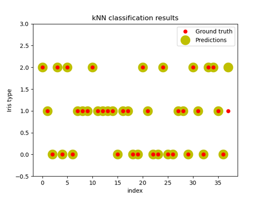
对测试集上数据预测的结果进行可视化输出，与真值进行对比

plt.figure(figsize=(10, 6))
plt.scatter(range(len(y_test)), y_test, c='red',s=80)
plt.scatter(range(len(y_test)), y_test_pred, c='green',s=20)
plt.title('kNN classification results')
plt.legend()
plt.show()

实验5 分类分析 - 图7

SVM训练

需要用的的数据集
iris.txt（使用时转换为.data格式）

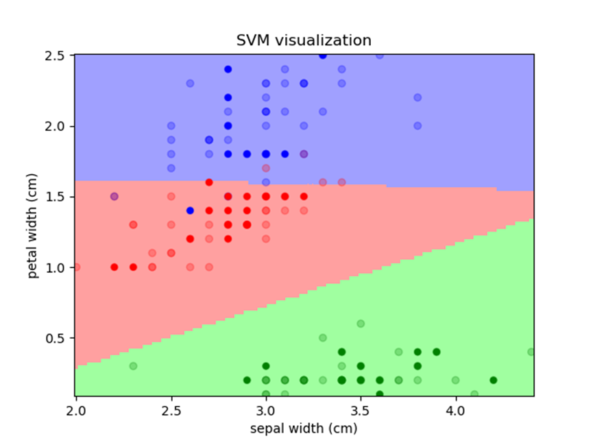
import numpy as np
from sklearn import svm
from sklearn import model_selection
import matplotlib.pyplot as plt
import matplotlib as mpl
#=============== 数据准备 ===============
file_path = "D:\DataAnalysis\iris.data"
# 该方法可将输入的字符串作为字典it 的键进行查询，输出对应的值
# 该方法就是相当于一个转换器，将数据中非浮点类型的字符串转化为浮点
def iris_type(s):
    it = {b'Iris-setosa':0, b'Iris-versicolor':1, b'Iris-virginica':2}
    return it[s]
# 加载data文件，类型为浮点，分隔符为逗号，对第四列也就是data 中的鸢尾花类别这一列的字符串转换为0-2 的浮点数
data = np.loadtxt(file_path, dtype=float, delimiter=',', converters={4:iris_type})
# print(data)
# 对data 矩阵进行分割，从第四列包括第四列开始后续所有列进行拆分
x, y = np.split(data, (4,), axis=1)
# 对x 矩阵进行切片，所有行都取，但只取前两列
x = x[:, 0:2]
print(x)
# 随机分配训练数据和测试数据，随机数种子为1，测试数据占比为0.3
data_train, data_test, tag_train, tag_test = model_selection.train_test_split(x, y, random_state=1, test_size=0.3)
#=============== 模型搭建 ===============
def classifier():
    clf = svm.SVC(C=0.5,                            # 误差惩罚系数，默认1
                  kernel='linear',                  # 线性核 kenrel='rbf':高斯核
                  decision_function_shape='ovr')    # 决策函数
    return clf
# 定义SVM（支持向量机）模型
clf = classifier()
#=============== 模型训练 ===============
def train(clf, x_train, y_train):
    clf.fit(x_train,            # 训练集特征向量
            y_train.ravel())    # 训练集目标值
# 训练SVM 模型
train(clf, data_train, tag_train)
#=============== 模型评估 ===============
def show_accuracy(a, b, tip):
    acc = a.ravel() == b.ravel()
    print('%s Accuracy:%.3f' % (tip, np.mean(acc)))
def print_accuracy(clf, x_train, y_train, x_test, y_test):
    # 分别打印训练集和测试集的准确率
    # score(x_train, y_train):表示输出x_train, y_train 在模型上的准确率
    print('training prediction:%.3f' % (clf.score(x_train, y_train)))
    print('test data prediction:%.3f' % (clf.score(x_test, y_test)))
    # 原始结果与预测结果进行对比
    # predict() 表示对x_train 样本进行预测，返回样本类别
    show_accuracy(clf.predict(x_train), y_train, 'training data')
    show_accuracy(clf.predict(x_test), y_test, 'testing data')
    # 计算决策函数的值，表示x到各分割平面的距离
    print('decision_function:\n', clf.decision_function(x_train))
print_accuracy(clf, data_train, tag_train, data_test, tag_test)
#=============== 模型可视化 ===============
def draw(clf, x):
    iris_feature = 'sepal length', 'sepal width', 'petal length', 'petal width'
    # 开始画图
    # 第0 列的范围
    x1_min, x1_max = x[:, 0].min(), x[:, 0].max()
    # 第1 列的范围
    x2_min, x2_max = x[:, 1].min(), x[:, 1].max()
    x1, x2 = np.mgrid[x1_min:x1_max:200j, x2_min:x2_max:200j]
    grid_test = np.stack((x1.flat, x2.flat), axis=1)
    print('grid_test:\n', grid_test)
    # 输出样本到决策面的距离
    z = clf.decision_function(grid_test)
    print('the distance to decision plane:\n', z)
    # 预测分类值
    grid_hat = clf.predict(grid_test)
    print('grid_hat:\n', grid_hat)
    grid_hat = grid_hat.reshape(x1.shape)
    cm_light = mpl.colors.ListedColormap(['#A0FFA0', '#FFA0A0', '#A0A0FF'])
    cm_dark = mpl.colors.ListedColormap(['g', 'r', 'b'])
    plt.pcolormesh(x1, x2, grid_hat, cmap=cm_light)
    # 样本点
    plt.scatter(x[:, 0], x[:, 1], c=np.squeeze(y), edgecolor='k', s=50, cmap=cm_dark)
    # 测试点
    plt.scatter(data_test[:, 0], data_test[:, 1], s=120, facecolor='none', zorder=10)
    plt.xlabel(iris_feature[0], fontsize=20)
    plt.ylabel(iris_feature[1], fontsize=20)
    plt.xlim(x1_min, x1_max)
    plt.ylim(x2_min, x2_max)
    plt.title('svm in iris data classification', fontsize=30)
    plt.grid()
    plt.show()
draw(clf, x)

[[5.1 3.5]
 [4.9 3. ]
 [4.7 3.2]
 [4.6 3.1]
 [5.  3.6]
 [5.4 3.9]
 [4.6 3.4]
 [5.  3.4]
 [4.4 2.9]
 [4.9 3.1]
 [5.4 3.7]
 [4.8 3.4]
 [4.8 3. ]
 [4.3 3. ]
 [5.8 4. ]
 [5.7 4.4]
 [5.4 3.9]
 [5.1 3.5]
 [5.7 3.8]
 [5.1 3.8]
 [5.4 3.4]
 [5.1 3.7]
 [4.6 3.6]
 [5.1 3.3]
 [4.8 3.4]
 [5.  3. ]
 [5.  3.4]
 [5.2 3.5]
 [5.2 3.4]
 [4.7 3.2]
 [4.8 3.1]
 [5.4 3.4]
 [5.2 4.1]
 [5.5 4.2]
 [4.9 3.1]
 [5.  3.2]
 [5.5 3.5]
 [4.9 3.1]
 [4.4 3. ]
 [5.1 3.4]
 [5.  3.5]
 [4.5 2.3]
 [4.4 3.2]
 [5.  3.5]
 [5.1 3.8]
 [4.8 3. ]
 [5.1 3.8]
 [4.6 3.2]
 [5.3 3.7]
 [5.  3.3]
 [7.  3.2]
 [6.4 3.2]
 [6.9 3.1]
 [5.5 2.3]
 [6.5 2.8]
 [5.7 2.8]
 [6.3 3.3]
 [4.9 2.4]
 [6.6 2.9]
 [5.2 2.7]
 [5.  2. ]
 [5.9 3. ]
 [6.  2.2]
 [6.1 2.9]
 [5.6 2.9]
 [6.7 3.1]
 [5.6 3. ]
 [5.8 2.7]
 [6.2 2.2]
 [5.6 2.5]
 [5.9 3.2]
 [6.1 2.8]
 [6.3 2.5]
 [6.1 2.8]
 [6.4 2.9]
 [6.6 3. ]
 [6.8 2.8]
 [6.7 3. ]
 [6.  2.9]
 [5.7 2.6]
 [5.5 2.4]
 [5.5 2.4]
 [5.8 2.7]
 [6.  2.7]
 [5.4 3. ]
 [6.  3.4]
 [6.7 3.1]
 [6.3 2.3]
 [5.6 3. ]
 [5.5 2.5]
 [5.5 2.6]
 [6.1 3. ]
 [5.8 2.6]
 [5.  2.3]
 [5.6 2.7]
 [5.7 3. ]
 [5.7 2.9]
 [6.2 2.9]
 [5.1 2.5]
 [5.7 2.8]
 [6.3 3.3]
 [5.8 2.7]
 [7.1 3. ]
 [6.3 2.9]
 [6.5 3. ]
 [7.6 3. ]
 [4.9 2.5]
 [7.3 2.9]
 [6.7 2.5]
 [7.2 3.6]
 [6.5 3.2]
 [6.4 2.7]
 [6.8 3. ]
 [5.7 2.5]
 [5.8 2.8]
 [6.4 3.2]
 [6.5 3. ]
 [7.7 3.8]
 [7.7 2.6]
 [6.  2.2]
 [6.9 3.2]
 [5.6 2.8]
 [7.7 2.8]
 [6.3 2.7]
 [6.7 3.3]
 [7.2 3.2]
 [6.2 2.8]
 [6.1 3. ]
 [6.4 2.8]
 [7.2 3. ]
 [7.4 2.8]
 [7.9 3.8]
 [6.4 2.8]
 [6.3 2.8]
 [6.1 2.6]
 [7.7 3. ]
 [6.3 3.4]
 [6.4 3.1]
 [6.  3. ]
 [6.9 3.1]
 [6.7 3.1]
 [6.9 3.1]
 [5.8 2.7]
 [6.8 3.2]
 [6.7 3.3]
 [6.7 3. ]
 [6.3 2.5]
 [6.5 3. ]
 [6.2 3.4]
 [5.9 3. ]]
training prediction:0.819
test data prediction:0.778
training data Accuracy:0.819
testing data Accuracy:0.778
decision_function:
 [[-0.5         1.20887337  2.29112663]
 [ 2.06328814 -0.0769677   1.01367956]
 [ 2.16674973  0.91702835 -0.08377808]
 [ 2.11427813  0.99765248 -0.11193061]
 [ 0.9925538   2.06392138 -0.05647518]
 [ 2.11742969  0.95255534 -0.06998503]
 [ 2.05615004 -0.041847    0.98569697]
 [-0.31866596  1.02685964  2.29180632]
 [-0.27166251  1.09150338  2.18015913]
 [-0.37827567  1.14260447  2.2356712 ]
 [-0.22150749  1.11104997  2.11045752]
 [-0.18331208  2.10066724  1.08264485]
 [-0.05444966  0.99927764  2.05517201]
 [-0.46977766  1.17853774  2.29123992]
 [-0.05760122  2.04437478  1.01322644]
 [ 2.1747228   0.93698124 -0.11170404]
 [-0.13315707  2.12021384  1.01294323]
 [-0.21752096  2.12102642  1.09649454]
 [ 2.11427813  0.99765248 -0.11193061]
 [ 2.16359817  0.96212549 -0.12572366]
 [-0.21038286  1.08590572  2.12447714]
 [ 2.21291822  0.9265985  -0.13951672]
 [-0.13399204  1.06514025  2.06885179]
 [-0.18016052  1.0555701   2.12459042]
 [-0.2334671   1.08112064  2.15234646]
 [-0.08782356  2.0747104   1.01311315]
 [-0.20324476  1.05078502  2.15245974]
 [-0.11489433  1.05994888  2.05494545]
 [ 2.17787437 -0.1081159   0.93024154]
 [-0.23578369  2.18129137  1.05449232]
 [-0.20639632  1.09588216  2.11051416]
 [-0.21038286  1.08590572  2.12447714]
 [-0.02969547  2.11420989  0.91548558]
 [-0.12685394  1.03001955  2.09683439]
 [-0.09496166  2.1098311   0.98513056]
 [ 2.10547008 -0.07737399  0.97190391]
 [ 2.11029159  0.98767604 -0.09796763]
 [ 2.20411017 -0.14842797  0.9443178 ]
 [-0.20324476  1.05078502  2.15245974]
 [ 2.19066895  0.97688701 -0.16755596]
 [-0.16022784  2.10545232  1.05477553]
 [-0.23661866  1.12621778  2.11040088]
 [-0.09579663  2.05475752  1.04103911]
 [ 2.11344315 -0.05742111  0.94397795]
 [ 2.10231852  0.96772315 -0.07004167]
 [-0.12203243  2.09506958  1.02696285]
 [ 2.11029159  0.98767604 -0.09796763]
 [-0.41248455  1.16296364  2.2495209 ]
 [-0.16820091  1.08549943  2.08270149]
 [-0.42045762  1.14301076  2.27744686]
 [-0.24857827  1.09628845  2.15228982]
 [-0.27796564  2.18169766  1.09626798]
 [-0.09264507  1.00966038  2.08298469]
 [-0.25339978  1.03123843  2.22216135]
 [-0.05361468  2.05435123  0.99926346]
 [ 2.15395516 -0.16797456  1.01401941]
 [-0.12203243  2.09506958  1.02696285]
 [ 2.06579305  1.08825305 -0.15404611]
 [-0.11007283  2.12499891  0.98507392]
 [-0.27166251  1.09150338  2.18015913]
 [ 2.13652739  0.94736397 -0.08389137]
 [-0.29789831  1.13181544  2.16608287]
 [ 2.15163856  0.93219616 -0.08383473]
 [ 2.1747228   0.93698124 -0.11170404]
 [-0.11174277  1.01485174  2.09689103]
 [-0.06872585  2.06951904  0.99920682]
 [-0.23745364  1.0711442   2.16630944]
 [ 2.12141623  0.96253178 -0.08394801]
 [ 2.1627632  -0.09294809  0.93018489]
 [-0.06557429  1.0244219   2.04115239]
 [ 2.16758471  0.97210193 -0.13968664]
 [-0.12203243  2.09506958  1.02696285]
 [ 2.1293893   0.98248467 -0.11187396]
 [-0.21038286  1.08590572  2.12447714]
 [ 2.01962457  1.0786829  -0.09830747]
 [ 2.18269588  0.95693412 -0.13963   ]
 [-0.16106282  1.05037873  2.11068408]
 [ 2.20976665  0.97169564 -0.1814623 ]
 [-0.03850351  2.03918342  0.9993201 ]
 [ 2.17555778  0.99205482 -0.1676126 ]
 [-0.11007283  2.12499891  0.98507392]
 [-0.07502898  2.15971332  0.91531566]
 [ 2.13254086  0.93738753 -0.06992839]
 [ 2.09518042  1.00284385 -0.09802427]
 [ 1.0045134   2.09385071 -0.09836411]
 [ 2.24314055  0.89626288 -0.13940344]
 [-0.09579663  2.05475752  1.04103911]
 [-0.14910321  1.08030806  2.06879515]
 [ 2.13652739  0.94736397 -0.08389137]
 [-0.2334671   1.08112064  2.15234646]
 [-0.07271239  2.05954259  1.0131698 ]
 [-0.2739791   2.1916741   1.082305  ]
 [-0.27564905  1.08152693  2.19412211]
 [-0.12203243  2.09506958  1.02696285]
 [ 2.06013657 -0.03187056  0.97173399]
 [ 2.07608272  1.00803521 -0.08411793]
 [-0.19443672  2.12581149  1.06862523]
 [-0.16421438  2.09547587  1.06873851]
 [-0.3440668   1.12224529  2.22182151]
 [-0.1180459   2.10504603  1.01299987]
 [-0.20240979  1.10585861  2.09655118]
 [-0.17617399  1.06554654  2.11062744]
 [-0.2477433   2.15136204  1.09638126]
 [-0.2334671   1.08112064  2.15234646]
 [ 2.11029159  0.98767604 -0.09796763]]
grid_test:
 [[4.3       2.       ]
 [4.3       2.0120603]
 [4.3       2.0241206]
 ...
 [7.9       4.3758794]
 [7.9       4.3879397]
 [7.9       4.4      ]]
the distance to decision plane:
 [[ 2.04663576  1.0980928  -0.14472856]
 [ 2.04808477  1.09663836 -0.14472313]
 [ 2.04953377  1.09518392 -0.1447177 ]
 ...
 [-0.21454554  0.96016146  2.25438408]
 [-0.21309653  0.95870702  2.25438951]
 [-0.21164753  0.95725258  2.25439495]]
grid_hat:
 [0. 0. 0. ... 2. 2. 2.]