一、调试处理

超参数

α：学习因子
β：动量梯度下降因子
β1,β2,ε：Adam算法参数
layers：神经网络层数
hidden units：各隐藏层神经元个数
learning rate decay：学习因子下降参数
mini-batch size：批量训练样本包含的样本个数

重要性

通常来说，学习因子αα是最重要的超参数，也是需要重点调试的超参数。动量梯度下降因子β、各隐藏层神经元个数#hidden units和mini-batch size的重要性仅次于αα。然后就是神经网络层数#layers和学习因子下降参数learning rate decay。最后，Adam算法的三个参数β1,β2,ε一般常设置为0.9，0.999和10−810−8，不需要反复调试。

调整

传统的机器学习，对每个超参数等间隔选取，然后，分别使用不同点对应的参数组合进行训练，最后根据验证集上的表现好坏，来选定最佳的参数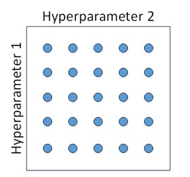


深度网络模型中，一般随机选取。因为每个参数的重要程度不同。例如上面对每个参数只有5种取值，下面这个则有25种情况。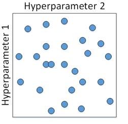

二、 Using an appropriate scale to pick hyperparameters

非均匀刻度尺

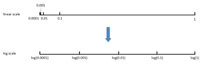
α、β
关于β的说明：假设β从0.9000变化为0.9005，那么1/1−β基本没有变化。但假设ββ从0.9990变化为0.9995，那么1/1−β前后差别1000。β越接近1，指数加权平均的个数越多，变化越大。所以对β接近1的区间，应该采集得更密集一些。

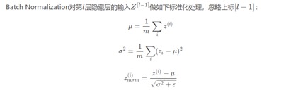
三、 Batch Normalization

标准化输入

在训练神经网络时，标准化输入可以提高训练的速度。方法是对训练数据集进行归一化的操作，即将原始数据减去其均值μ后，再除以其方差σ2。

batch norm

一般进一步处理

Normalizing inputs使所有输入的均值为0，方差为1。而Batch Normalization可使各隐藏层输入的均值和方差为任意值。实际上，从激活函数的角度来说，如果各隐藏层的输入均值在靠近0的区域即处于激活函数的线性区域，这样不利于训练好的非线性神经网络，得到的模型效果也不会太好。

四、 Why does Batch Norm work

如果发生covariate shift，因为batch norm的作用，隐藏层的输出均值和方差仍不变，则其他参数会更加稳定，模型在其他样本上也会有不错的表现。
从另一个方面来说，Batch Norm也起到轻微的正则化（regularization）效果。具体表现在：

• 每个mini-batch都进行均值为0，方差为1的归一化操作
• 每个mini-batch中，对各个隐藏层的Z[l]添加了随机噪声，效果类似于Dropout
• mini-batch越小，正则化效果越明显

  五、 softmax回归

  介绍

  对于二分类问题，网络的输出层只有一个神经单元，输出值表示预测输出为正类的概率， 则判断为正类， 则判断为负类。
  对于多分类问题，用C表示种类个数，神经网络中输出层就有C个神经元，其中每个神经元的输出依次对应属于该类的概率。为了处理多分类问题，我们一般使用Softmax回归模型。其激活函数如下：
  

  损失函数

  

六、深度学习框架

• Caffe
• Keras
• CNTK
• DL4J
• Lasagne
• mxnet
• PaddlePaddle
• Tensorflow
• Theano
• Torch

选择框架的标准：

• ease of programming
• running speed
• truly open

七、编程作业

• create placeholder

def create_placeholders(n_x, n_y):
    """
    Creates the placeholders for the tensorflow session.
    Arguments:
    n_x -- scalar, size of an image vector (num_px * num_px = 64 * 64 * 3 = 12288)
    n_y -- scalar, number of classes (from 0 to 5, so -> 6)
    Returns:
    X -- placeholder for the data input, of shape [n_x, None] and dtype "float"
    Y -- placeholder for the input labels, of shape [n_y, None] and dtype "float"
    Tips:
    - You will use None because it let's us be flexible on the number of examples you will for the placeholders.
      In fact, the number of examples during test/train is different.
    """
    ### START CODE HERE ### (approx. 2 lines)
    X = tf.placeholder(tf.float32, [n_x, None], name="X")
    Y = tf.placeholder(tf.float32, [n_y, None], name='Y')
    ### END CODE HERE ###
    return X, Y

• initializing the parameters

# GRADED FUNCTION: initialize_parameters
def initialize_parameters():
    """
    Initializes parameters to build a neural network with tensorflow. The shapes are:
                        W1 : [25, 12288]
                        b1 : [25, 1]
                        W2 : [12, 25]
                        b2 : [12, 1]
                        W3 : [6, 12]
                        b3 : [6, 1]
    Returns:
    parameters -- a dictionary of tensors containing W1, b1, W2, b2, W3, b3
    """
    tf.set_random_seed(1)                   # so that your "random" numbers match ours
    ### START CODE HERE ### (approx. 6 lines of code)
    W1 = tf.get_variable("W1", [25,12288], initializer = tf.contrib.layers.xavier_initializer(seed = 1))
    b1 = tf.get_variable("b1",[25,1],initializer=tf.zeros_initializer())
    W2 = tf.get_variable("W2", [12, 25], initializer = tf.contrib.layers.xavier_initializer(seed=1))
    b2 = tf.get_variable("b2", [12, 1], initializer = tf.zeros_initializer())
    W3 = tf.get_variable("W3", [6, 12], initializer = tf.contrib.layers.xavier_initializer(seed=1))
    b3 = tf.get_variable("b3", [6, 1], initializer = tf.zeros_initializer())
    ### END CODE HERE ###
    parameters = {"W1": W1,
                  "b1": b1,
                  "W2": W2,
                  "b2": b2,
                  "W3": W3,
                  "b3": b3}
    return parameters

• forward propagation in tensorflow

# GRADED FUNCTION: forward_propagation
def forward_propagation(X, parameters):
    """
    Implements the forward propagation for the model: LINEAR -> RELU -> LINEAR -> RELU -> LINEAR -> SOFTMAX
    Arguments:
    X -- input dataset placeholder, of shape (input size, number of examples)
    parameters -- python dictionary containing your parameters "W1", "b1", "W2", "b2", "W3", "b3"
                  the shapes are given in initialize_parameters
    Returns:
    Z3 -- the output of the last LINEAR unit
    """
    # Retrieve the parameters from the dictionary "parameters" 
    W1 = parameters['W1']
    b1 = parameters['b1']
    W2 = parameters['W2']
    b2 = parameters['b2']
    W3 = parameters['W3']
    b3 = parameters['b3']
    ### START CODE HERE ### (approx. 5 lines)              # Numpy Equivalents:
    Z1 = tf.add(tf.matmul(W1,X),b1)                                              # Z1 = np.dot(W1, X) + b1
    A1 = tf.nn.relu(Z1)                                              # A1 = relu(Z1)
    Z2 = tf.add(tf.matmul(W2,A1),b2)                                             # Z2 = np.dot(W2, a1) + b2s
    A2 = tf.nn.relu(Z2)                                              # A2 = relu(Z2)
    Z3 = tf.add(tf.matmul(W3,A2),b3)                                              # Z3 = np.dot(W3,Z2) + b3
    ### END CODE HERE ###
    return Z3

• compute cost

# GRADED FUNCTION: compute_cost 
def compute_cost(Z3, Y):
    """
    Computes the cost
    Arguments:
    Z3 -- output of forward propagation (output of the last LINEAR unit), of shape (6, number of examples)
    Y -- "true" labels vector placeholder, same shape as Z3
    Returns:
    cost - Tensor of the cost function
    """
    # to fit the tensorflow requirement for tf.nn.softmax_cross_entropy_with_logits(...,...)
    logits = tf.transpose(Z3)
    labels = tf.transpose(Y)
    ### START CODE HERE ### (1 line of code)
    cost = tf.reduce_mean(tf.nn.softmax_cross_entropy_with_logits(logits=logits,labels=labels))
    ### END CODE HERE ###
    return cost

• backward propagation & parameter updates

#For instance, for gradient descent the optimizer would be:
optimizer = tf.train.GradientDescentOptimizer(learning_rate = learning_rate).minimize(cost)
#To make the optimization you would do:
_ , c = sess.run([optimizer, cost], feed_dict={X: minibatch_X, Y: minibatch_Y})