1. 目的

实现高尔夫球的运动轨迹计算与推测

2. 步骤

识别到高尔夫球
可以画出或者标定出高尔夫球的运动轨迹
根据起飞角、抛物线公式来预测高尔夫球的运动距离

3. 方案

3.1 识别高尔夫球

3.1.1 根据高尔夫球颜色

定义高尔夫球的HSV色域空间范围
resize后的效果：

这一步除了尺寸有变化，其它都和原图一样。

高斯滤波后的效果：

滤掉了高频噪音，看着变模糊了。

转换到HSV色域后的效果：

二值化后的效果：

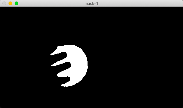
腐蚀和膨胀后的效果：

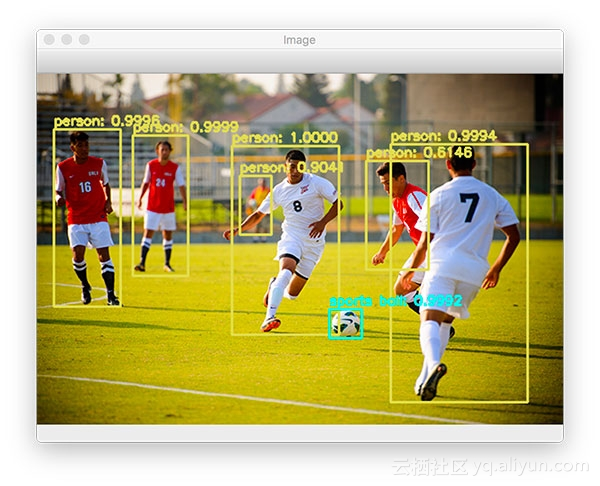
3.1.2 使用yolov3目标检测来检测高尔夫球

3.2 画出或者标定出高尔夫球的运动轨迹

    # 寻找轮廓，不同opencv的版本cv2.findContours返回格式有区别，所以调用了一下imutils.grab_contours做了一些兼容性处理
    cnts = cv2.findContours(mask.copy(), cv2.RETR_EXTERNAL, cv2.CHAIN_APPROX_SIMPLE)
    cnts = imutils.grab_contours(cnts)
    center = None
    # only proceed if at least one contour was found
    if len(cnts) > 0:
        # find the largest contour in the mask, then use it to compute the minimum enclosing circle
        # and centroid
        c = max(cnts, key=cv2.contourArea)
        ((x, y), radius) = cv2.minEnclosingCircle(c)
        M = cv2.moments(c)
        # 对于01二值化的图像，m00即为轮廓的面积, 一下公式用于计算中心距
        center = (int(M["m10"] / M["m00"]), int(M["m01"] / M["m00"]))
        # only proceed if the radius meets a minimum size
        if radius > 10:
            # draw the circle and centroid on the frame, then update the list of tracked points
            cv2.circle(frame, (int(x), int(y)), int(radius), (0, 255, 255), 2)
            cv2.circle(frame, center, 5, (0, 0, 255), -1)
        pts.appendleft(center)
    for i in range(1, len(pts)):
        # if either of the tracked points are None, ignore them
        if pts[i - 1] is None or pts[i] is None:
            continue
        # compute the thickness of the line and draw the connecting line
        thickness = int(np.sqrt(args["buffer"] / float(i + 1)) * 2.5)
        cv2.line(frame, pts[i - 1], pts[i], (0, 0, 255), thickness)
    cv2.imshow("Frame", frame)

3.3 根据起飞角、抛物线公式来预测高尔夫球的运动距离

将离散的轨迹坐标拟合为曲线，从而预测运动参数方法/函数
使用最小二乘法拟合运动抛物线 ```python
二次函数的标准形式
def func(params, x): a, b, c = params return a x x + b * x + c

误差函数，即拟合曲线所求的值与实际值的差

def error(params, x, y): return func(params, x) - y

对参数求解

def slovePara(): p0 = [10, 10, 10]

p0 = [0.1,-0.01,100]

Para = leastsq(error, p0, args=(X, Y)) return Para 输出最后的结果 def solution(): Para = slovePara() a, b, c = Para[0] print(“a=”,a,” b=”,b,” c=”,c) print (“cost:” + str(Para[1])) print (“求解的曲线是:”) print(“y=”+str(round(a,2))+”xx+”+str(round(b,2))+”x+”+str(c))
plt.figure(figsize=(8,6))#创建一个 8 6 点（point）的图 plt.scatter(X, Y, color=”green”, label=”sample data”, linewidth=2) ##画出样本数据画拟合曲线 x=np.linspace(-10,50,100) ##在-10-50直接画100个连续点 y=axx+b*x+c ##函数式 plt.plot(x,y,color=”red”,label=”solution line”,linewidth=2)

plt.title(“python实现最小二乘法曲线拟合”)

plt.legend() #绘制图例看拟合效果 plt.show() solution() ```

共享

高尔夫球运动轨迹计算与推测技术方案