回溯测试

When I first started trading, I thought trading was all about coming up with clever strategies and then,
just to be sure, testing them on historical data.

This is the complete opposite of how strategies are actually developed.
First, you collect and cleanse your data. Then you use the development back tester to identify potentially profitable correlations（关联） and behaviors in the data. After you rank these from most promising to least, you validate the best ones using an implementation backtester. This is a long and somewhat tedious process, but gives you a much higher probability of making money once the strategy goes live.

In this section, we explore how you can validate and develop a quantitative strategy using a historical dataset. We also look at what you are trying to accomplish with the backtesting, and some of the mistakes developers commonly make when attempting to validate a strategy.
Lastly, we will highlight the differences between development backtesting models that you create to
evaluate multiple strategies on multiple datasets and implementation models that are used to retest the strategies that are already good candidates for live trading.

First, we will explore how developers validated quantitative strategy that has been created using a historical dataset. A classic backtest starts with a time series of historical asset prices that is divided into two series: a training series A and a testing series B. You train your model using data from the training window, and then you apply that model on data in the testing window.
This allows you to compute the performance of your model with data that was not used in its creation.
Backtesting is part of an iterative process in which you first use a series of price data to fit a mathematical model of predictable price patterns and behaviors.
You then use this model of patterns and behaviors to design a quantitative strategy that will allow you to initiate orders to buy and sell the asset and also to set stop loss orders to manage position risk.
You optimize a strategy to maximize the profit within your risk tolerance, from trading the price series in period A. We will talk later in the course about the details of how to develop these strategies.
But for now, we will just focus on how these strategies are validated. It wouldn’t make sense for you to validate a strategy with the same data you use to create it. So you reserve part of your historical data series to test your strategy out of sample. Backtesting at its simplest is just running your strategy on
the price data from period B, and seeing if you can replicate the performance of your strategy achieved in period A. If performance in the backtest is negative or extremely weak, you abandon the strategy and start over. If it is positive but does not meet your minimum risk return requirements, you might be tempted to tweak your strategy and retest it on period B data. Although tweaking seems reasonable,
you run the risk of overfitting your model to the data. If the strategy’s performance in period B
meets or even better exceeds period A results, then you are ready to either go live with your strategy,
which is a bit risky, or more commonly paper trade the strategy for a while with live data and then gradually commit trading capital if it continues to generate Alpha.

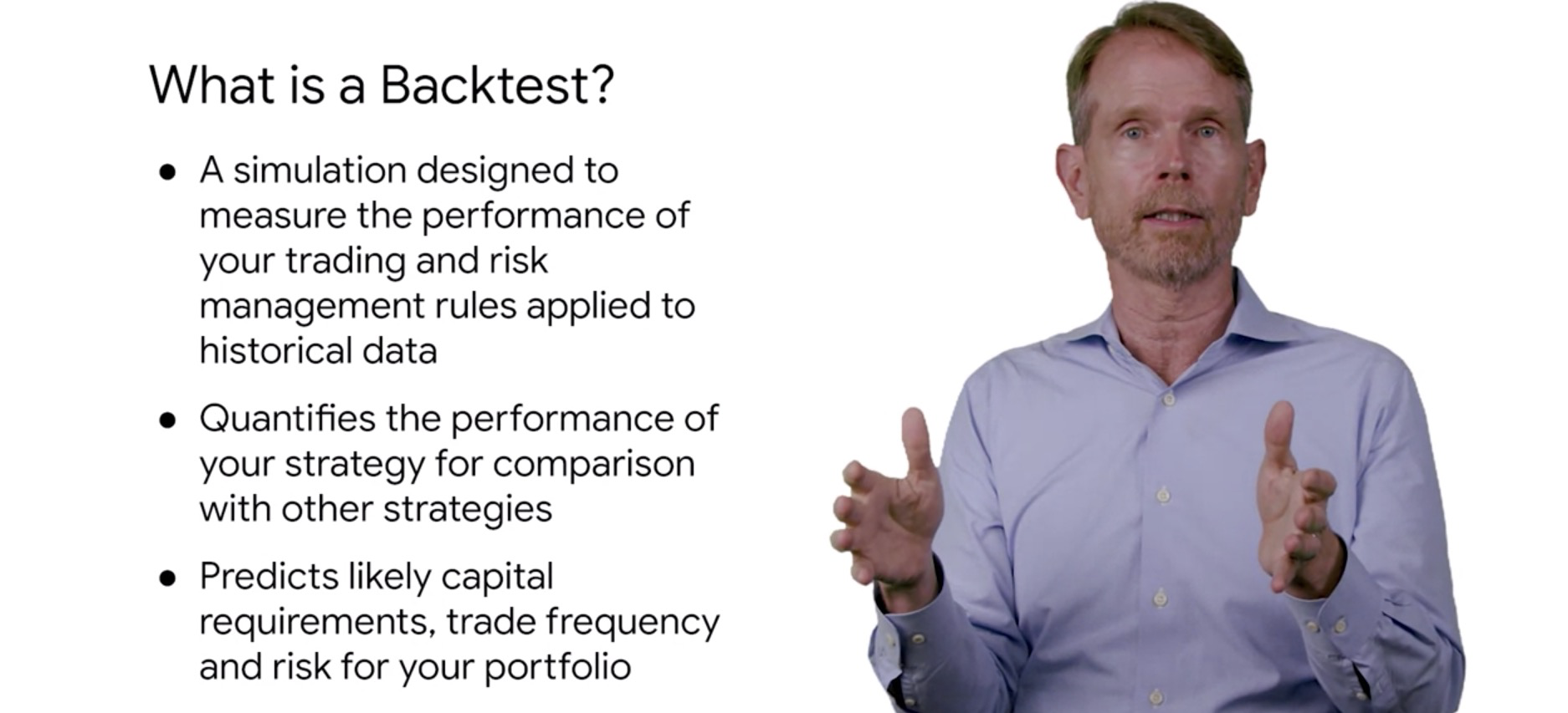
A backtest is a simulation of the performance you would have achieved if you had traded your strategy during a particular historical period(回溯测试是对在特定历史时期内交易策略所能达到的绩效的模拟。
). It includes trading and risk management rules to simulate a live trading environment.
You can then compare those performance to that of other strategies implemented on the same asset.
Last week, backtest give you an estimate of the capital you will need, risk involved, and transaction costs you could incur if you decide to live trade a strategy. Another type of task that we commonly use for time series models that have been built using machine learning methods is the sliding window backtest.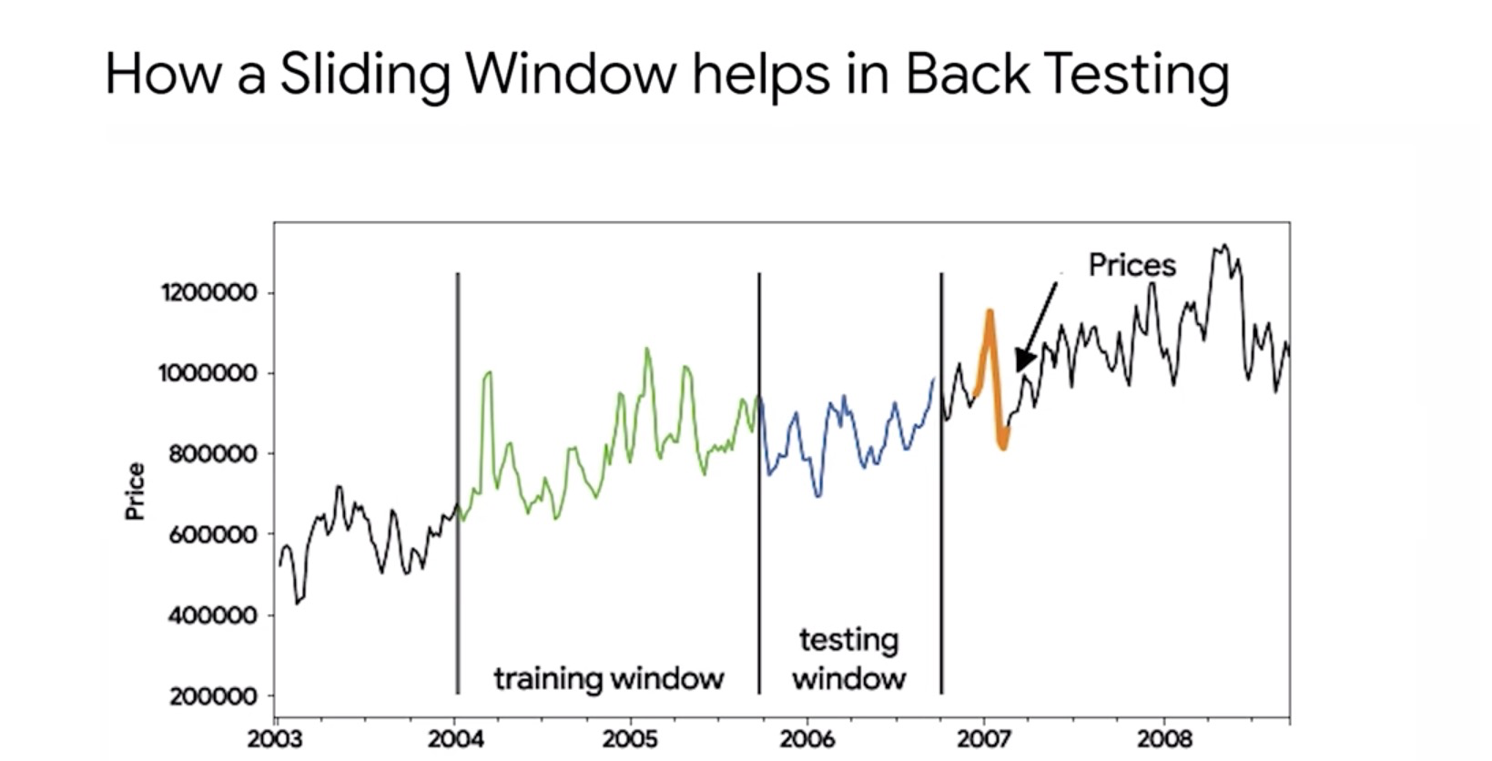

In a sliding window test, the whole dataset is divided into a series of adjoining pairs of training and testing windows. You train a model using a training window and then apply that model on
the adjoining testing window to compute performance through the first run.
For the next run, you slide the training window to the new set of training records and repeat
this process until you’ve used all of the training windows. With this technique, you can calculate
an average performance metric across the entire dataset. Performance metrics you derived through
sliding window validation are generally more robust than split validation techniques that we discussed earlier. Notice how the training window or the testing window moved together across the entire time series of data. This allows your strategy to be modeled and tested on almost the entire dataset rather than just half of it.