一、pytorch 基础练习
1. 定义数据
一般定义数据使用torch.Tensor , tensor的意思是张量,是数字各种形式的总称
import torch# 可以是一个数x = torch.tensor(666)print(x)

#可以是一维数组(向量)x = torch.tensor([1, 2, 3, 4, 5, 6])print(x)

#可以是二维数组(矩阵)x = torch.ones(2, 3)print(x)

# 可以是任意维度的数组(张量)x = torch.ones(2, 3, 4)print(x)

Tensor支持各种各样类型的数据,包括:
torch.float32, torch.float64, torch.float16, torch.uint8, torch.int8, torch.int16, torch.int32, torch.int64 。这里不过多描述。
创建Tensor有多种方法,包括:ones, zeros, eye, arange, linspace, rand, randn, normal, uniform, randperm, 使用的时候可以在线搜,下面主要通过代码展示。
# 创建一个空张量x = torch.empty(5, 3)print(x)

# 创建一个随机初始化的张量x = torch.rand(5, 3)print(x)

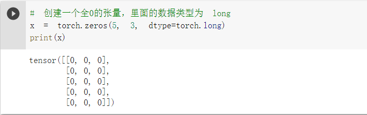
# 创建一个全0的张量,里面的数据类型为 longx = torch.zeros(5, 3, dtype=torch.long)print(x)
# 基于现有的tensor,创建一个新tensor,# 从而可以利用原有的tensor的dtype,device,size之类的属性信息y = x.new_ones(5, 3) #tensor new_* 方法,利用原来tensor的dtype,deviceprint(y)

z = torch.randn_like(x, dtype=torch.float) # 利用原来的tensor的大小,但是重新定义了dtypeprint(z)

2. 定义操作
凡是用Tensor进行各种运算的,都是Function
最终,还是需要用Tensor来进行计算的,计算无非是
- 基本运算,加减乘除,求幂求余
- 布尔运算,大于小于,最大最小
- 线性运算,矩阵乘法,求模,求行列式
基本运算包括: abs/sqrt/div/exp/fmod/pow ,及一些三角函数 cos/ sin/ asin/ atan2/ cosh,及 ceil/round/floor/trunc 等具体在使用的时候可以百度一下
布尔运算包括: gt/lt/ge/le/eq/ne,topk, sort, max/min
线性计算包括: trace, diag, mm/bmm,t,dot/cross,inverse,svd 等
不再多说,需要使用的时候百度一下即可。下面用具体的代码案例来学习。
# 创建一个 2x4 的tensorm = torch.Tensor([[2, 5, 6, 4],[1, 9, 0, 8]])print(m.size(0), m.size(1), m.size(), sep=' -- ') #sep设置字符串之间的分隔符

# 返回 m 中元素的数量print(m.numel())

# 返回第0行,第2列的数print(m[0][2])

# 返回第1列的全部元素print(m[:, 1])

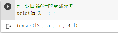
# 返回第0行的全部元素print(m[0, :])
# Create tensor of numbers from 1 to 5# 注意这里结果是1到4,没有5v = torch.arange(1, 5)print(v)

# Scalar product#先查看数据类型print(m.dtype)print(v.dtype)

#数据类型转换后 进行矩阵相乘m = m.long()print(m.dtype)

# Calculated by 1*2 + 2*5 + 3*6 + 4*4m[0, :] @ v

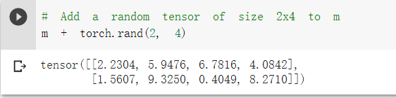
# Add a random tensor of size 2x4 to mm + torch.rand(2, 4)
# 转置,由 2x4 变为 4x2print(m.t())# 使用 transpose 也可以达到相同的效果,具体使用方法可以百度print(m.transpose(0, 1))

# returns a 1D tensor of steps equally spaced points between start=3, end=8 and steps=20torch.linspace(3, 8, 20)

from matplotlib import pyplot as plt# matlabplotlib 只能显示numpy类型的数据,下面展示了转换数据类型,然后显示# 注意 randn 是生成均值为 0, 方差为 1 的随机数# 下面是生成 1000 个随机数,并按照 100 个 bin 统计直方图plt.hist(torch.randn(1000).numpy(), 100);

# 当数据非常非常多的时候,正态分布会体现的非常明显plt.hist(torch.randn(10**6).numpy(), 100);

# 创建两个 1x4 的tensora = torch.tensor([[1, 2, 3, 4]])b = torch.tensor([[5, 6, 7, 8]])# 在 0 方向拼接 (即在 Y 方各上拼接), 会得到 2x4 的矩阵print(torch.cat((a, b), 0))

# 在 1 方向拼接 (即在 X 方各上拼接), 会得到 1x8 的矩阵print(torch.cat((a, b), 1))

二、螺旋数据分布
本次的代码教程里解决 sprial classification 问题,教程有配套的文字版讲解理论,地址为:https://atcold.github.io/pytorch-Deep-Learning/chapters/02-3/ 基础一般的同学可以适当看看理论
下载绘图函数到本地。(画点的过程中要用到里面的一些函数)
!wget https://raw.githubusercontent.com/Atcold/pytorch-Deep-Learning/master/res/plot_lib.py
引入基本的库,然后初始化重要参数
import randomimport torchfrom torch import nn, optimimport mathfrom IPython import displayfrom plot_lib import plot_data, plot_model, set_default# 因为colab是支持GPU的,torch 将在 GPU 上运行device = torch.device("cuda:0" if torch.cuda.is_available() else "cpu")print('device: ', device)# 初始化随机数种子。神经网络的参数都是随机初始化的,# 不同的初始化参数往往会导致不同的结果,当得到比较好的结果时我们通常希望这个结果是可以复现的,# 因此,在pytorch中,通过设置随机数种子也可以达到这个目的seed = 12345random.seed(seed)torch.manual_seed(seed)N = 1000 # 每类样本的数量D = 2 # 每个样本的特征维度C = 3 # 样本的类别H = 100 # 神经网络里隐层单元的数量
device: cuda:0
初始化 X 和 Y。 X 可以理解为特征矩阵,Y可以理解为样本标签。 结合代码可以看到,X的为一个 N x C 行, D 列的矩阵。C 类样本,每类样本是 N个,所以是 N*C 行。每个样本的特征维度是2,所以是 2列。
在 python 中,调用 zeros 类似的函数,第一个参数是 y方向的,即矩阵的行;第二个参数是 x方向的,即矩阵的列,大家得注意下,不要搞反了。下面结合代码看看 3000个样本的特征是如何初始化的。
X = torch.zeros(N * C, D).to(device)Y = torch.zeros(N * C, dtype=torch.long).to(device)for c in range(C):index = 0t = torch.linspace(0, 1, N) # 在[0,1]间均匀的取10000个数,赋给t# 下面的代码不用理解太多,总之是根据公式计算出三类样本(可以构成螺旋形)# torch.randn(N) 是得到 N 个均值为0,方差为 1 的一组随机数,注意要和 rand 区分开inner_var = torch.linspace( (2*math.pi/C)*c, (2*math.pi/C)*(2+c), N) + torch.randn(N) * 0.2# 每个样本的(x,y)坐标都保存在 X 里# Y 里存储的是样本的类别,分别为 [0, 1, 2]for ix in range(N * c, N * (c + 1)):X[ix] = t[index] * torch.FloatTensor((math.sin(inner_var[index]), math.cos(inner_var[index])))Y[ix] = cindex += 1print("Shapes: ")print("X: ", X.size())print("Y: ", Y.size())
Shapes:
X: torch.Size([3000, 2])
Y: torch.Size([3000])
# visualise the dataplot_data(X, Y)

1.构建线性模型分类
learning_rate = 1e-3lambda_l2 = 1e-5# nn 包用来创建线性模型# 每一个线性模型都包含 weight 和 biasmodel = nn.Sequential(nn.Linear(D, H),nn.Linear(H, C))model.to(device) # 把模型放到GPU上# nn 包含多种不同的损失函数,这里使用的是交叉熵(cross entropy loss)损失函数criterion = torch.nn.CrossEntropyLoss()# 这里使用 optim 包进行随机梯度下降(stochastic gradient descent)优化optimzer = torch.optim.SGD(model.parameters(), lr=learning_rate, weight_decay=lambda_l2)# 开始训练for t in range(1000):# 把数据输入模型,得到预测结果y_pred = model(X)# 计算损失和准确率loss = criterion(y_pred, Y)score, predicted = torch.max(y_pred, 1)acc = (Y == predicted).sum().float() / len(Y)print('[EPOCH]: %i, [LOSS]: %.6f, [ACCURACY]: %.3f' % (t, loss.item(), acc))display.clear_output(wait=True)# 反向传播前把梯度置 0optimzer.zero_grad()# 反向传播优化loss.backward()# 更新全部参数optimzer.step()
[EPOCH]: 999, [LOSS]: 0.873033, [ACCURACY]: 0.499
这里对上面的一些关键函数进行说明:
使用 print(y_pred.shape) 可以看到模型的预测结果,为[3000, 3]的矩阵。每个样本的预测结果为3个,保存在 y_pred 的一行里。值最大的一个,即为预测该样本属于的类别
score, predicted = torch.max(y_pred, 1) 是沿着第二个方向(即X方向)提取最大值。最大的那个值存在 score 中,所在的位置(即第几列的最大)保存在 predicted 中。下面代码把第10行的情况输出,供解释说明
此外,大家可以看到,每一次反向传播前,都要把梯度清零,这个在知乎上有一个回答,大家可以参考:https://www.zhihu.com/question/303070254
print(y_pred.shape)print(y_pred[10, :])print(score[10])print(predicted[10])
torch.Size([3000, 3])
tensor([-0.1599, -0.1676, -0.1469], grad_fn=
tensor(-0.1469, grad_fn=
tensor(2)
# Plot trained modelprint(model)plot_model(X, Y, model)
Sequential(
(0): Linear(in_features=2, out_features=100, bias=True)
(1): Linear(in_features=100, out_features=3, bias=True)
)
上面使用 print(model) 把模型输出,可以看到有两层:
- 第一层输入为 2(因为特征维度为主2),输出为 100;
- 第二层输入为 100 (上一层的输出),输出为 3(类别数)
从上面图示可以看出,线性模型的准确率最高只能达到 50% 左右,对于这样复杂的一个数据分布,线性模型难以实现准确分类。
2.构建两层神经网络分类
# 这里可以看到,和上面模型不同的是,在两层之间加入了一个 ReLU 激活函数model = nn.Sequential(nn.Linear(D, H),nn.ReLU(),nn.Linear(H, C))model.to(device)# 下面的代码和之前是完全一样的,这里不过多叙述criterion = torch.nn.CrossEntropyLoss()optimizer = torch.optim.Adam(model.parameters(), lr=learning_rate, weight_decay=lambda_l2) # built-in L2# 训练模型,和之前的代码是完全一样的for t in range(1000):y_pred = model(X)loss = criterion(y_pred, Y)score, predicted = torch.max(y_pred, 1)acc = ((Y == predicted).sum().float() / len(Y))print("[EPOCH]: %i, [LOSS]: %.6f, [ACCURACY]: %.3f" % (t, loss.item(), acc))display.clear_output(wait=True)# zero the gradients before running the backward pass.optimizer.zero_grad()# Backward pass to compute the gradientloss.backward()# Update paramsoptimizer.step()
[EPOCH]: 999, [LOSS]: 0.168418, [ACCURACY]: 0.952
# Plot trained model
print(model)
plot_model(X, Y, model)
Sequential(
0): Linear(in_features=2, out_features=100, bias=True)
(1): ReLU() (2): Linear(in_features=100, out_features=3, bias=True)
)
可以看到,在两层神经网络里加入 ReLU 激活函数以后,分类的准确率得到了显著提高。

若有收获,就点个赞吧
0 人点赞
