
一、MobileNet V1
本文提出了一类有效的模型称为移动和嵌入式视觉应用程序的MobileNet。MobileNet基于一种流线型的架构,使用深度可分离的卷积来构建轻量级的深度神经网络。
深度可分离卷积就是将普通卷积拆分成为一个深度卷积和一个逐点卷积。
深度卷积:
与标准卷积网络不一样的是,我们将卷积核拆分成为但单通道形式,在不改变输入特征图像的深度的情况下,对每一通道进行卷积操作,这样就得到了和输入特征图通道数一致的输出特征图。如图:
输入12×12×3的特征图,经过5×5×1×3的深度卷积之后,得到了8×8×3的输出特征图。输入个输出的维度是不变的3。这样就会有一个问题,通道数太少,特征图的维度太少

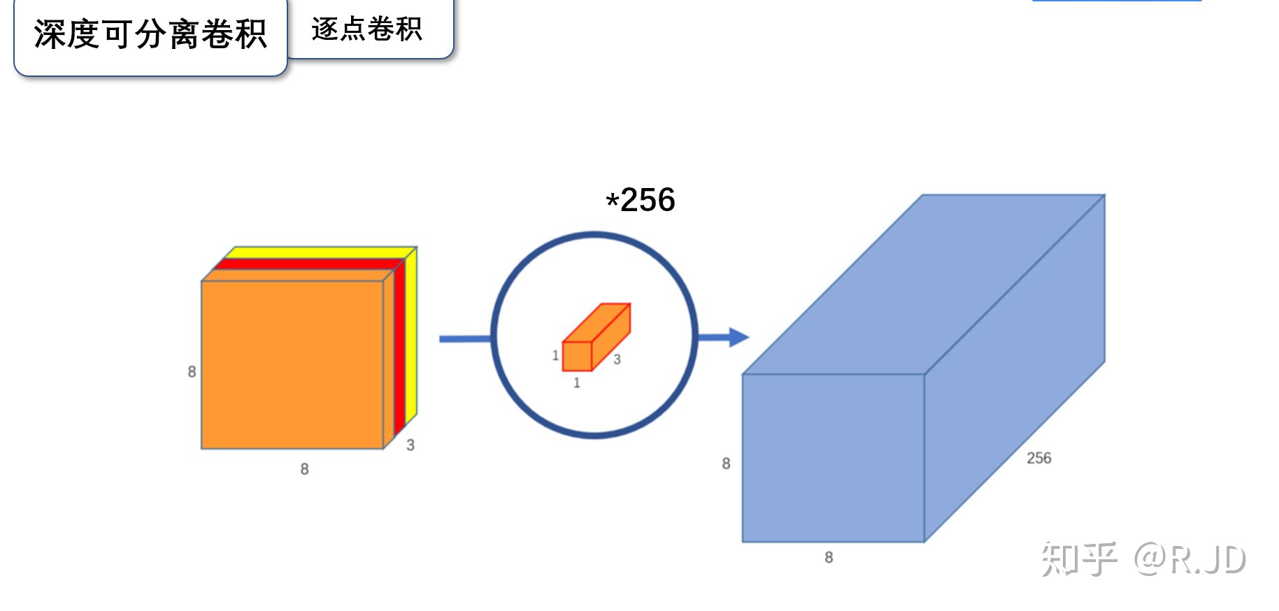
逐点卷积:
逐点卷积就是1×1卷积。主要作用就是对特征图进行升维和降维,如图:
在深度卷积的过程中,我们得到了8×8×3的输出特征图,我们用256个1×1×3的卷积核对输入特征图进行卷积操作,输出的特征图和标准的卷积操作一样都是8×8×256了。
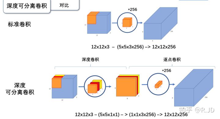
标准卷积与深度可分离卷积的过程对比如下:
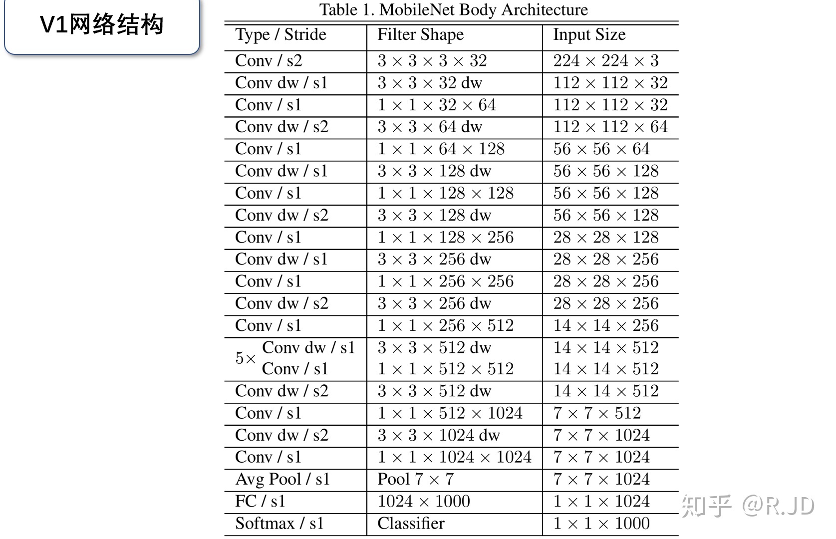
V1网络结构
MobileNet 可分离卷积部分的代码:
import torchimport torch.nn as nnimport torch.nn.functional as Fimport torchvisionimport torchvision.transforms as transformsimport matplotlib.pyplot as pltimport numpy as npimport torch.optim as optimclass Block(nn.Module):'''Depthwise conv + Pointwise conv'''def __init__(self, in_planes, out_planes, stride=1):super(Block, self).__init__()# Depthwise 卷积,3*3 的卷积核,分为 in_planes,即各层单独进行卷积self.conv1 = nn.Conv2d(in_planes, in_planes, kernel_size=3, stride=stride, padding=1, groups=in_planes, bias=False)self.bn1 = nn.BatchNorm2d(in_planes)# Pointwise 卷积,1*1 的卷积核self.conv2 = nn.Conv2d(in_planes, out_planes, kernel_size=1, stride=1, padding=0, bias=False)self.bn2 = nn.BatchNorm2d(out_planes)def forward(self, x):out = F.relu(self.bn1(self.conv1(x)))out = F.relu(self.bn2(self.conv2(out)))return out
创建DataLoader:
device = torch.device("cuda:0" if torch.cuda.is_available() else "cpu")transform_train = transforms.Compose([transforms.RandomCrop(32, padding=4),transforms.RandomHorizontalFlip(),transforms.ToTensor(),transforms.Normalize((0.4914, 0.4822, 0.4465), (0.2023, 0.1994, 0.2010))])transform_test = transforms.Compose([transforms.ToTensor(),transforms.Normalize((0.4914, 0.4822, 0.4465), (0.2023, 0.1994, 0.2010))])trainset = torchvision.datasets.CIFAR10(root='./data', train=True, download=True, transform=transform_train)testset = torchvision.datasets.CIFAR10(root='./data', train=False, download=True, transform=transform_test)trainloader = torch.utils.data.DataLoader(trainset, batch_size=128, shuffle=True, num_workers=2)testloader = torch.utils.data.DataLoader(testset, batch_size=128, shuffle=False, num_workers=2)

创建MobileNetV1网络:
32×32×3 ==>
32×32×32 ==> 32×32×64 ==> 16×16×128 ==> 16×16×128 ==>
8×8×256 ==> 8×8×256 ==> 4×4×512 ==> 4×4×512 ==>
2×2×1024 ==> 2×2×1024
接下来为均值 pooling ==> 1×1×1024
最后全连接到 10个输出节点
class MobileNetV1(nn.Module):# (128,2) means conv planes=128, stride=2cfg = [(64,1), (128,2), (128,1), (256,2), (256,1), (512,2), (512,1),(1024,2), (1024,1)]def __init__(self, num_classes=10):super(MobileNetV1, self).__init__()self.conv1 = nn.Conv2d(3, 32, kernel_size=3, stride=1, padding=1, bias=False)self.bn1 = nn.BatchNorm2d(32)self.layers = self._make_layers(in_planes=32)self.linear = nn.Linear(1024, num_classes)def _make_layers(self, in_planes):layers = []for x in self.cfg:out_planes = x[0]stride = x[1]layers.append(Block(in_planes, out_planes, stride))in_planes = out_planesreturn nn.Sequential(*layers)def forward(self, x):out = F.relu(self.bn1(self.conv1(x)))out = self.layers(out)out = F.avg_pool2d(out, 2)out = out.view(out.size(0), -1)out = self.linear(out)return out
实例化网络:
net = MobileNetV1().to(device)
criterion = nn.CrossEntropyLoss()
optimizer = optim.Adam(net.parameters(), lr=0.001)
模型训练:
for epoch in range(10): # 重复多轮训练
for i, (inputs, labels) in enumerate(trainloader):
inputs = inputs.to(device)
labels = labels.to(device)
# 优化器梯度归零
optimizer.zero_grad()
# 正向传播 + 反向传播 + 优化
outputs = net(inputs)
loss = criterion(outputs, labels)
loss.backward()
optimizer.step()
# 输出统计信息
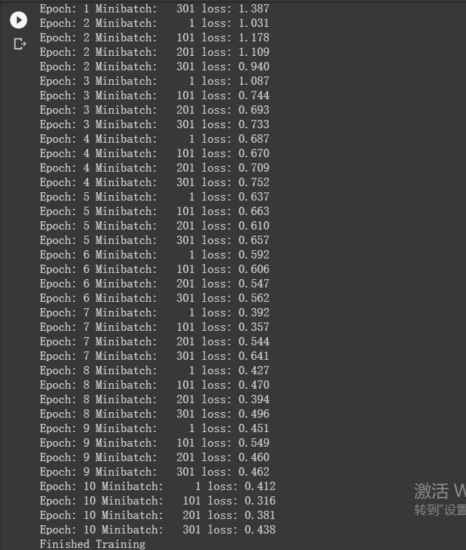
if i % 100 == 0:
print('Epoch: %d Minibatch: %5d loss: %.3f' %(epoch + 1, i + 1, loss.item()))
print('Finished Training')

模型测试:
correct = 0
total = 0

for data in testloader:
    images, labels = data
    images, labels = images.to(device), labels.to(device)
    outputs = net(images)
    _, predicted = torch.max(outputs.data, 1)
    total += labels.size(0)
    correct += (predicted == labels).sum().item()

print('Accuracy of the network on the 10000 test images: %.2f %%' % (
    100 * correct / total))

网络放弃了部分准确性,高效压缩了存储和计算量。
二、MobileNet V2
MobileNetV2可以提高移动模型在多个任务和基准上的最佳性能,也可以跨越不同型号大小的范围。
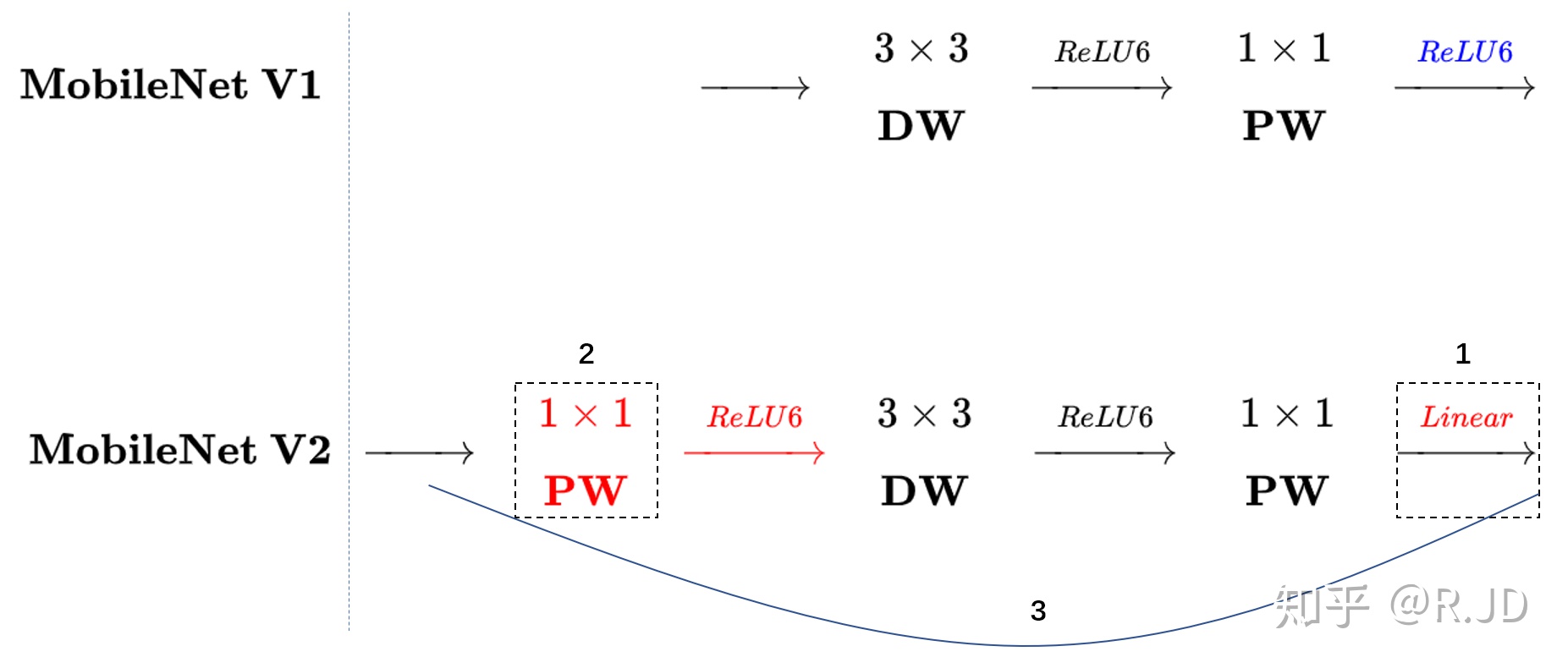
Linear bottleneck
把最后的ReLU6换成Linear,作者将这个部分称之为linear bottleneck
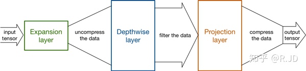
Expansion layer
深度卷积本身没有改变通道的能力,来的是多少通道输出就是多少通道。如果来的通道很少的话,DW深度卷积只能在低维度上工作,这样效果并不会很好,所以我们要“扩张”通道。既然我们已经知道PW逐点卷积也就是1×1卷积可以用来升维和降维,那就可以在DW深度卷积之前使用PW卷积进行升维(升维倍数为t,t=6),再在一个更高维的空间中进行卷积操作来提取特征:

也就是说,不管输入通道数是多少,经过第一个PW逐点卷积升维之后,深度卷积都是在相对的更高6倍维度上进行工作。
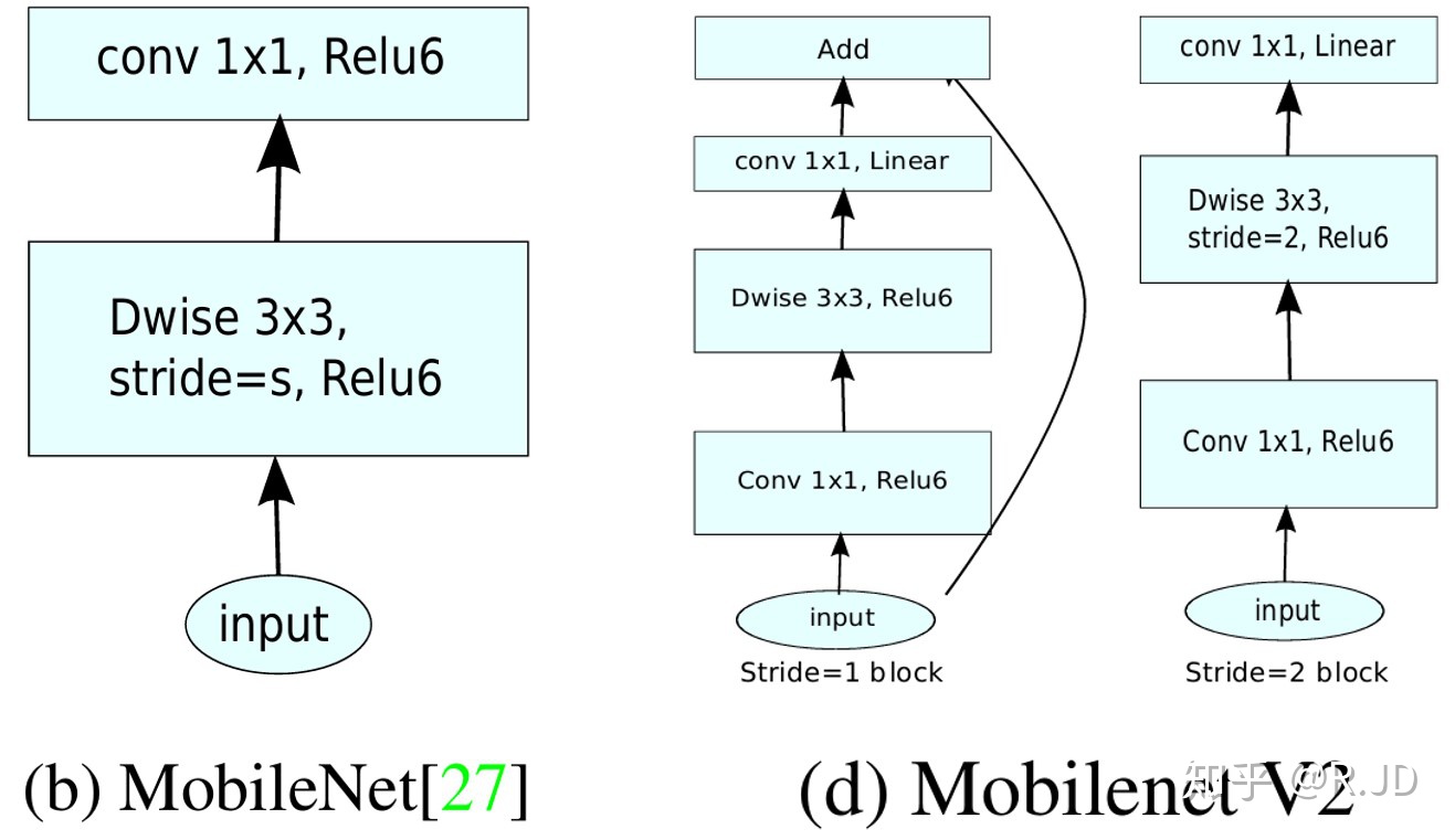
Inverted residuals
回顾V1的网络结构,我们发现V1很像是一个直筒型的VGG网络。我们想像Resnet一样复用我们的特征,所以我们引入了shortcut结构,这样V2的block就是如下图形式:
对比一下V1和V2:

可以发现,都采用了 1×1 -> 3 ×3 -> 1 × 1 的模式,以及都使用Shortcut结构。但是不同点呢:
- ResNet 先降维 (0.25倍)、卷积、再升维。
- MobileNetV2 则是 先升维 (6倍)、卷积、再降维。
刚好V2的block刚好与Resnet的block相反,作者将其命名为Inverted residuals。就是论文名中的Inverted residuals。
V2的block:
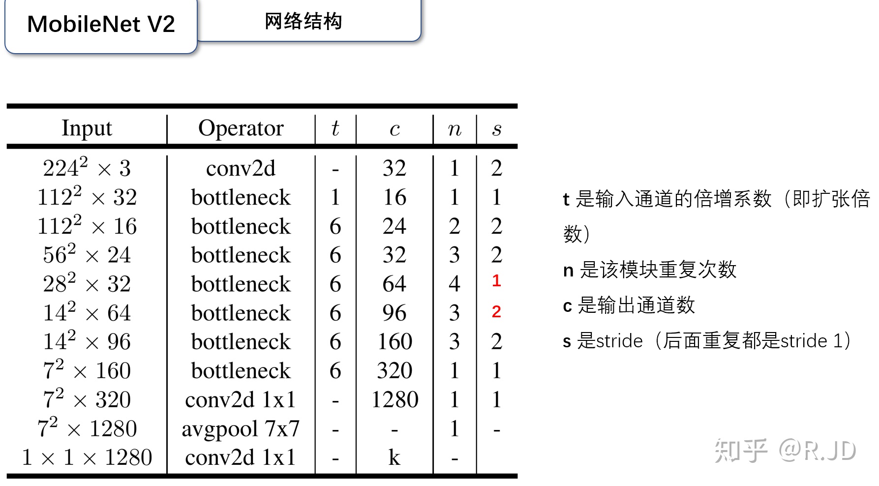
V2的网络结构
Inverted residual block 部分的代码:
import torch
import torch.nn as nn
import torch.nn.functional as F
import torchvision
import torchvision.transforms as transforms
import matplotlib.pyplot as plt
import numpy as np
import torch.optim as optim

class Block(nn.Module):
    '''expand + depthwise + pointwise'''
    def __init__(self, in_planes, out_planes, expansion, stride):
        super(Block, self).__init__()
        self.stride = stride
        # 通过 expansion 增大 feature map 的数量
        planes = expansion * in_planes
        self.conv1 = nn.Conv2d(in_planes, planes, kernel_size=1, stride=1, padding=0, bias=False)
        self.bn1 = nn.BatchNorm2d(planes)
        self.conv2 = nn.Conv2d(planes, planes, kernel_size=3, stride=stride, padding=1, groups=planes, bias=False)
        self.bn2 = nn.BatchNorm2d(planes)
        self.conv3 = nn.Conv2d(planes, out_planes, kernel_size=1, stride=1, padding=0, bias=False)
        self.bn3 = nn.BatchNorm2d(out_planes)

        # 步长为 1 时,如果 in 和 out 的 feature map 通道不同,用一个卷积改变通道数
        if stride == 1 and in_planes != out_planes:
            self.shortcut = nn.Sequential(
                nn.Conv2d(in_planes, out_planes, kernel_size=1, stride=1, padding=0, bias=False),
                nn.BatchNorm2d(out_planes))
        # 步长为 1 时,如果 in 和 out 的 feature map 通道相同,直接返回输入
        if stride == 1 and in_planes == out_planes:
            self.shortcut = nn.Sequential()

    def forward(self, x):
        out = F.relu(self.bn1(self.conv1(x)))
        out = F.relu(self.bn2(self.conv2(out)))
        out = self.bn3(self.conv3(out))
        # 步长为1,加 shortcut 操作
        if self.stride == 1:
            return out + self.shortcut(x)
        # 步长为2,直接输出
        else:
            return out
创建MobileNetV2网络:
class MobileNetV2(nn.Module):
    # (expansion, out_planes, num_blocks, stride)
    cfg = [(1,  16, 1, 1),
           (6,  24, 2, 1),
           (6,  32, 3, 2),
           (6,  64, 4, 2),
           (6,  96, 3, 1),
           (6, 160, 3, 2),
           (6, 320, 1, 1)]

    def __init__(self, num_classes=10):
        super(MobileNetV2, self).__init__()
        self.conv1 = nn.Conv2d(3, 32, kernel_size=3, stride=1, padding=1, bias=False)
        self.bn1 = nn.BatchNorm2d(32)
        self.layers = self._make_layers(in_planes=32)
        self.conv2 = nn.Conv2d(320, 1280, kernel_size=1, stride=1, padding=0, bias=False)
        self.bn2 = nn.BatchNorm2d(1280)
        self.linear = nn.Linear(1280, num_classes)

    def _make_layers(self, in_planes):
        layers = []
        for expansion, out_planes, num_blocks, stride in self.cfg:
            strides = [stride] + [1]*(num_blocks-1)
            for stride in strides:
                layers.append(Block(in_planes, out_planes, expansion, stride))
                in_planes = out_planes
        return nn.Sequential(*layers)

    def forward(self, x):
        out = F.relu(self.bn1(self.conv1(x)))
        out = self.layers(out)
        out = F.relu(self.bn2(self.conv2(out)))
        out = F.avg_pool2d(out, 4)
        out = out.view(out.size(0), -1)
        out = self.linear(out)
        return out
创建DataLoader:
device = torch.device("cuda:0" if torch.cuda.is_available() else "cpu")

transform_train = transforms.Compose([
    transforms.RandomCrop(32, padding=4),
    transforms.RandomHorizontalFlip(),
    transforms.ToTensor(),
    transforms.Normalize((0.4914, 0.4822, 0.4465), (0.2023, 0.1994, 0.2010))])

transform_test = transforms.Compose([
    transforms.ToTensor(),
    transforms.Normalize((0.4914, 0.4822, 0.4465), (0.2023, 0.1994, 0.2010))])

trainset = torchvision.datasets.CIFAR10(root='./data', train=True,  download=True, transform=transform_train)
testset  = torchvision.datasets.CIFAR10(root='./data', train=False, download=True, transform=transform_test)

trainloader = torch.utils.data.DataLoader(trainset, batch_size=128, shuffle=True, num_workers=2)
testloader = torch.utils.data.DataLoader(testset, batch_size=128, shuffle=False, num_workers=2)
实例化网络:
net = MobileNetV2().to(device)
criterion = nn.CrossEntropyLoss()
optimizer = optim.Adam(net.parameters(), lr=0.001)
模型训练:
for epoch in range(10):
  for i, (inputs, labels) in enumerate(trainloader):
    inputs = inputs.to(device)
    labels = labels.to(device)
    optimizer.zero_grad()
    outputs = net(inputs)
    loss = criterion(outputs, labels)
    loss.backward()
    optimizer.step()
    if i % 100 == 0:
      print('Epoch: %d Minibatch: %5d loss: %.3f' %(epoch + 1, i + 1, loss.item()))

print('Finished Training')
模型测试:
correct = 0
total = 0

for data in testloader:
  images, labels = data
  images, labels = images.to(device), labels.to(device)
  outputs = net(images)
  _, predicted = torch.max(outputs.data, 1)
  total += labels.size(0)
  correct += (predicted == labels).sum().item()

print('Accuracy of the network on the 10000 test images: %.2f %%' % (
    100 * correct / total))

三、HybridSN
高光谱图像(HSI)分类广泛应用于遥感图像分析。卷积神经网络(CNN)是最常用的基于深度学习的视觉数据处理方法之一。本文提出了一个混合光谱CNN (hybrid spectral CNN, HybridSN)用于HSI分类。
网络结构

定义HybridSN 类
class_num = 16

class HybridSN(nn.Module):
  def __init__(self, num_classes=16):
    super(HybridSN, self).__init__()
    # conv1:(1, 30, 25, 25), 8个 7x3x3 的卷积核 ==>(8, 24, 23, 23)
    self.conv1 = nn.Conv3d(1, 8, (7, 3, 3))
    # conv2:(8, 24, 23, 23), 16个 5x3x3 的卷积核 ==>(16, 20, 21, 21)
    self.conv2 = nn.Conv3d(8, 16, (5, 3, 3))
    # conv3:(16, 20, 21, 21),32个 3x3x3 的卷积核 ==>(32, 18, 19, 19)
    self.conv3 = nn.Conv3d(16, 32, (3, 3, 3))
    # conv3_2d (576, 19, 19),64个 3x3 的卷积核 ==>((64, 17, 17)
    self.conv3_2d = nn.Conv2d(576, 64, (3,3))
    # 全连接层(256个节点)
    self.dense1 =  nn.Linear(18496,256)
    # 全连接层(128个节点)
    self.dense2 =  nn.Linear(256,128)
    # 最终输出层(16个节点)
    self.out = nn.Linear(128, num_classes)
    #  Dropout(0.4)
    self.drop = nn.Dropout(p=0.4)
    self.soft = nn.LogSoftmax(dim=1)
    # 激活函数ReLU
    self.relu = nn.ReLU()
  def forward(self, x):
    out = self.relu(self.conv1(x))
    out = self.relu(self.conv2(out))
    out = self.relu(self.conv3(out))
    # 进行二维卷积,因此把前面的 32*18 reshape 一下,得到 (576, 19, 19)
    out = out.view(-1, out.shape[1] * out.shape[2], out.shape[3], out.shape[4])
    out = self.relu(self.conv3_2d(out))
    # flatten 操作,变为 18496 维的向量,
    out = out.view(out.size(0), -1)
    out = self.dense1(out)
    out = self.drop(out)
    out = self.dense2(out)
    out = self.drop(out)
    out = self.out(out)
    out = self.soft(out)
    return out
随机输入,测试网络结构是否通
x = torch.randn(1, 1, 30, 25, 25)
net = HybridSN()
y = net(x)
print(y.shape)

创建数据集:
首先对高光谱数据实施PCA降维;然后创建 keras 方便处理的数据格式;然后随机抽取 10% 数据做为训练集,剩余的做为测试集。
首先定义基本函数:
# 对高光谱数据 X 应用 PCA 变换
def applyPCA(X, numComponents):
    newX = np.reshape(X, (-1, X.shape[2]))
    pca = PCA(n_components=numComponents, whiten=True)
    newX = pca.fit_transform(newX)
    newX = np.reshape(newX, (X.shape[0], X.shape[1], numComponents))
    return newX

# 对单个像素周围提取 patch 时,边缘像素就无法取了,因此,给这部分像素进行 padding 操作
def padWithZeros(X, margin=2):
    newX = np.zeros((X.shape[0] + 2 * margin, X.shape[1] + 2* margin, X.shape[2]))
    x_offset = margin
    y_offset = margin
    newX[x_offset:X.shape[0] + x_offset, y_offset:X.shape[1] + y_offset, :] = X
    return newX

# 在每个像素周围提取 patch ,然后创建成符合 keras 处理的格式
def createImageCubes(X, y, windowSize=5, removeZeroLabels = True):
    # 给 X 做 padding
    margin = int((windowSize - 1) / 2)
    zeroPaddedX = padWithZeros(X, margin=margin)
    # split patches
    patchesData = np.zeros((X.shape[0] * X.shape[1], windowSize, windowSize, X.shape[2]))
    patchesLabels = np.zeros((X.shape[0] * X.shape[1]))
    patchIndex = 0
    for r in range(margin, zeroPaddedX.shape[0] - margin):
        for c in range(margin, zeroPaddedX.shape[1] - margin):
            patch = zeroPaddedX[r - margin:r + margin + 1, c - margin:c + margin + 1]
            patchesData[patchIndex, :, :, :] = patch
            patchesLabels[patchIndex] = y[r-margin, c-margin]
            patchIndex = patchIndex + 1
    if removeZeroLabels:
        patchesData = patchesData[patchesLabels>0,:,:,:]
        patchesLabels = patchesLabels[patchesLabels>0]
        patchesLabels -= 1
    return patchesData, patchesLabels

def splitTrainTestSet(X, y, testRatio, randomState=345):
    X_train, X_test, y_train, y_test = train_test_split(X, y, test_size=testRatio, random_state=randomState, stratify=y)
    return X_train, X_test, y_train, y_test
下面读取并创建数据集:
# 地物类别
class_num = 16
X = sio.loadmat('Indian_pines_corrected.mat')['indian_pines_corrected']
y = sio.loadmat('Indian_pines_gt.mat')['indian_pines_gt']

# 用于测试样本的比例
test_ratio = 0.90
# 每个像素周围提取 patch 的尺寸
patch_size = 25
# 使用 PCA 降维,得到主成分的数量
pca_components = 30

print('Hyperspectral data shape: ', X.shape)
print('Label shape: ', y.shape)

print('\n... ... PCA tranformation ... ...')
X_pca = applyPCA(X, numComponents=pca_components)
print('Data shape after PCA: ', X_pca.shape)

print('\n... ... create data cubes ... ...')
X_pca, y = createImageCubes(X_pca, y, windowSize=patch_size)
print('Data cube X shape: ', X_pca.shape)
print('Data cube y shape: ', y.shape)

print('\n... ... create train & test data ... ...')
Xtrain, Xtest, ytrain, ytest = splitTrainTestSet(X_pca, y, test_ratio)
print('Xtrain shape: ', Xtrain.shape)
print('Xtest  shape: ', Xtest.shape)

# 改变 Xtrain, Ytrain 的形状,以符合 keras 的要求
Xtrain = Xtrain.reshape(-1, patch_size, patch_size, pca_components, 1)
Xtest  = Xtest.reshape(-1, patch_size, patch_size, pca_components, 1)
print('before transpose: Xtrain shape: ', Xtrain.shape)
print('before transpose: Xtest  shape: ', Xtest.shape)

# 为了适应 pytorch 结构,数据要做 transpose
Xtrain = Xtrain.transpose(0, 4, 3, 1, 2)
Xtest  = Xtest.transpose(0, 4, 3, 1, 2)
print('after transpose: Xtrain shape: ', Xtrain.shape)
print('after transpose: Xtest  shape: ', Xtest.shape)


""" Training dataset"""
class TrainDS(torch.utils.data.Dataset):
    def __init__(self):
        self.len = Xtrain.shape[0]
        self.x_data = torch.FloatTensor(Xtrain)
        self.y_data = torch.LongTensor(ytrain)
    def __getitem__(self, index):
        # 根据索引返回数据和对应的标签
        return self.x_data[index], self.y_data[index]
    def __len__(self):
        # 返回文件数据的数目
        return self.len

""" Testing dataset"""
class TestDS(torch.utils.data.Dataset):
    def __init__(self):
        self.len = Xtest.shape[0]
        self.x_data = torch.FloatTensor(Xtest)
        self.y_data = torch.LongTensor(ytest)
    def __getitem__(self, index):
        # 根据索引返回数据和对应的标签
        return self.x_data[index], self.y_data[index]
    def __len__(self):
        # 返回文件数据的数目
        return self.len

# 创建 trainloader 和 testloader
trainset = TrainDS()
testset  = TestDS()
train_loader = torch.utils.data.DataLoader(dataset=trainset, batch_size=128, shuffle=True, num_workers=2)
test_loader  = torch.utils.data.DataLoader(dataset=testset,  batch_size=128, shuffle=False, num_workers=2)

开始训练:
# 使用GPU训练,可以在菜单 "代码执行工具" -> "更改运行时类型" 里进行设置
device = torch.device("cuda:0" if torch.cuda.is_available() else "cpu")
# 网络放到GPU上
net = HybridSN().to(device)
criterion = nn.CrossEntropyLoss()
optimizer = optim.Adam(net.parameters(), lr=0.0005)
# 开始训练
total_loss = 0
for epoch in range(100):
for i, (inputs, labels) in enumerate(train_loader):
inputs = inputs.to(device)
labels = labels.to(device)
# 优化器梯度归零
optimizer.zero_grad()
# 正向传播 + 反向传播 + 优化
outputs = net(inputs)
loss = criterion(outputs, labels)
loss.backward()
optimizer.step()
total_loss += loss.item()
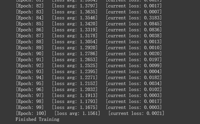
print('[Epoch: %d] [loss avg: %.4f] [current loss: %.4f]' %(epoch + 1, total_loss/(epoch+1), loss.item()))
print('Finished Training')
模型测试:
count = 0
# 模型测试
for inputs, _ in test_loader:
    inputs = inputs.to(device)
    outputs = net(inputs)
    outputs = np.argmax(outputs.detach().cpu().numpy(), axis=1)
    if count == 0:
        y_pred_test =  outputs
        count = 1
    else:
        y_pred_test = np.concatenate( (y_pred_test, outputs) )

# 生成分类报告
classification = classification_report(ytest, y_pred_test, digits=4)
print(classification)


测试结果波动,原因是加入了dropout层。
在训练时应当指定当前是训练模式:model.train();在测试时应当指定是测试模式:model.eval()。
参考文献:

若有收获,就点个赞吧
0 人点赞
