setup.py(设置算法库)
from setuptools import setupfrom setuptools import find_packagessetup(name='pygcn',version='0.1',description='Graph Convolutional Networks in PyTorch',author='Thomas Kipf',author_email='thomas.kipf@gmail.com',url='https://tkipf.github.io',download_url='https://github.com/tkipf/pygcn',license='MIT',install_requires=['numpy','torch','scipy'],package_data={'pygcn': ['README.md']},packages=find_packages())
utils.py
import numpy as npimport scipy.sparse as spimport torchimport scipy.io as sioimport randomfrom sklearn import preprocessingdef encode_onehot(labels):classes = set(labels) # set() 函数创建一个无序不重复元素集# enumerate()函数生成序列,带有索引i和值c。# 这一句将string类型的label变为onehot编码的label,建立映射关系classes_dict = {c: np.identity(len(classes))[i, :] for i, c inenumerate(classes)}# map() 会根据提供的函数对指定序列做映射。# 这一句将string类型的label替换为onehot编码的labellabels_onehot = np.array(list(map(classes_dict.get, labels)),dtype=np.int32)# 返回int类型的labelreturn labels_onehot'''数据读取'''# 更改路径。由../改为C:\Users\73416\PycharmProjects\PyGCNdef load_data(path="C:/Users/73416/PycharmProjects/PyGCN_Visualization/data/cora/", dataset="cora"):"""Load citation network dataset (cora only for now)"""print('Loading {} dataset...'.format(dataset))'''cora.content 介绍:cora.content共有2708行,每一行代表一个样本点,即一篇论文。每一行由三部分组成:是论文的编号,如31336;论文的词向量,一个有1433位的二进制;论文的类别,如Neural_Networks。总共7种类别(label)第一个是论文编号,最后一个是论文类别,中间是自己的信息(feature)''''''读取feature和label'''# 以字符串形式读取数据集文件:各自的信息。idx_features_labels = np.genfromtxt("{}{}.content".format(path, dataset),dtype=np.dtype(str))# csr_matrix:Compressed Sparse Row marix,稀疏np.array的压缩# idx_features_labels[:, 1:-1]表明跳过论文编号和论文类别,只取自己的信息(feature of node)features = sp.csr_matrix(idx_features_labels[:, 1:-1], dtype=np.float32)# idx_features_labels[:, -1]表示只取最后一个,即论文类别,得到的返回值为int类型的labellabels = encode_onehot(idx_features_labels[:, -1])# build graph# idx_features_labelsidx_features_labels[:, 0]表示取论文编号idx = np.array(idx_features_labels[:, 0], dtype=np.int32)# 通过建立论文序号的序列,得到论文序号的字典idx_map = {j: i for i, j in enumerate(idx)}edges_unordered = np.genfromtxt("{}{}.cites".format(path, dataset),dtype=np.int32)# 进行一次论文序号的映射# 论文编号没有用,需要重新的其进行编号(从0开始),然后对原编号进行替换。# 所以目的是把离散的原始的编号,变成0 - 2707的连续编号edges = np.array(list(map(idx_map.get, edges_unordered.flatten())),dtype=np.int32).reshape(edges_unordered.shape)# coo_matrix():系数矩阵的压缩。分别定义有那些非零元素,以及各个非零元素对应的row和col,最后定义稀疏矩阵的shape。adj = sp.coo_matrix((np.ones(edges.shape[0]), (edges[:, 0], edges[:, 1])),shape=(labels.shape[0], labels.shape[0]),dtype=np.float32)# build symmetric adjacency matrixadj = adj + adj.T.multiply(adj.T > adj) - adj.multiply(adj.T > adj)# feature和adj归一化features = normalize(features)adj = normalize(adj + sp.eye(adj.shape[0]))# train set, validation set, test set的分组。idx_train = range(140)idx_val = range(200, 500)idx_test = range(500, 1500)# 数据类型转tensorfeatures = torch.FloatTensor(np.array(features.todense()))labels = torch.LongTensor(np.where(labels)[1])adj = sparse_mx_to_torch_sparse_tensor(adj)idx_train = torch.LongTensor(idx_train)idx_val = torch.LongTensor(idx_val)idx_test = torch.LongTensor(idx_test)# 返回数据return adj, features, labels, idx_train, idx_val, idx_testdef load_data2(dataset_source):data = sio.loadmat("../data/{}.mat".format(dataset_source))features = data["Attributes"]adj = data["Network"]labels = data["Label"]nb_nodes = features.shape[0]ft_size = features.shape[1]lb = preprocessing.LabelBinarizer()labels = lb.fit_transform(labels)# adj = adj + adj.T.multiply(adj.T > adj) - adj.multiply(adj.T > adj)# features = normalize(features)adj = normalize(adj + sp.eye(adj.shape[0]))# features = preprocessing.normalize(features, norm='l2', axis=0)node_perm = np.random.permutation(labels.shape[0])num_train = int(0.05 * adj.shape[0])num_val = int(0.1 * adj.shape[0])idx_train = node_perm[:num_train]idx_val = node_perm[num_train:num_train + num_val]idx_test = node_perm[num_train + num_val:]features = torch.FloatTensor(np.array(features.todense()))labels = torch.LongTensor(np.where(labels)[1])adj = sparse_mx_to_torch_sparse_tensor(adj)idx_train = torch.LongTensor(idx_train)idx_val = torch.LongTensor(idx_val)idx_test = torch.LongTensor(idx_test)return adj, features, labels, idx_train, idx_val, idx_testdef normalize(mx):"""Row-normalize sparse matrix"""rowsum = np.array(mx.sum(1)) # (2708, 1)r_inv = np.power(rowsum, -1).flatten() # (2708,)r_inv[np.isinf(r_inv)] = 0. # 处理除数为0导致的infr_mat_inv = sp.diags(r_inv)mx = r_mat_inv.dot(mx)return mxdef accuracy(output, labels):preds = output.max(1)[1].type_as(labels)correct = preds.eq(labels).double()correct = correct.sum()return correct / len(labels)def sparse_mx_to_torch_sparse_tensor(sparse_mx):"""Convert a scipy sparse matrix to a torch sparse tensor."""sparse_mx = sparse_mx.tocoo().astype(np.float32)indices = torch.from_numpy(np.vstack((sparse_mx.row, sparse_mx.col)).astype(np.int64))values = torch.from_numpy(sparse_mx.data)shape = torch.Size(sparse_mx.shape)return torch.sparse.FloatTensor(indices, values, shape)
标签编码函数:encode_onehot(labels)
def encode_onehot(labels):classes = set(labels) # set() 函数创建一个无序不重复元素集# enumerate()函数生成序列,带有索引i和值c。# 这一句将string类型的label变为int类型的label,建立映射关系classes_dict = {c: np.identity(len(classes))[i, :] for i, c inenumerate(classes)}# map() 会根据提供的函数对指定序列做映射。# 这一句将string类型的label替换为int类型的labellabels_onehot = np.array(list(map(classes_dict.get, labels)),dtype=np.int32)# 返回int类型的labelreturn labels_onehot
该函数用于改变标签labels的编码格式。将离散的字符串类型的labels,使用onehot编码,得到onehot编码形式的labels。
onehot编码,又称“独热编码”。其实就是用N位状态寄存器编码N个状态。每个状态都有独立的寄存器位,且这些寄存器位中只有一位有效,说白了就是只能有一个状态。
更多关于onehot编码的细节,参见博客:[数据预处理] onehot编码:是什么,为什么,怎么样。
对于Cora数据集的labels,处理前是离散的字符串标签:
[Genetic_Algorithms’, ‘Probabilistic_Methods’, ‘Reinforcement_Learning’, ‘Neural_Networks’, ‘Theory’, ‘Case_Based’, ‘Rule_Learning’ ]
对labels进行onehot编码后的结果如下:
# 'Genetic_Algorithms': array([1., 0., 0., 0., 0., 0., 0.]),# 'Probabilistic_Methods': array([0., 1., 0., 0., 0., 0., 0.]),# 'Reinforcement_Learning': array([0., 0., 1., 0., 0., 0., 0.]),# 'Neural_Networks': array([0., 0., 0., 1., 0., 0., 0.]),# 'Theory': array([0., 0., 0., 0., 1., 0., 0.]),# 'Case_Based': array([0., 0., 0., 0., 0., 1., 0.]),# 'Rule_Learning': array([0., 0., 0., 0., 0., 0., 1.])}
这里再附上使用onehot编码对Cora数据集的样本标签进行编码的Demo:
from pygcn.utils import encode_onehotimport numpy as np'''labels的onehot编码,前后结果对比'''# 读取原始数据集path="../data/cora/"dataset = "cora"idx_features_labels = np.genfromtxt("{}{}.content".format(path, dataset),dtype=np.dtype(str))RawLabels=idx_features_labels[:, -1]print("原始论文类别(label):\n",RawLabels)# ['Neural_Networks' 'Rule_Learning' 'Reinforcement_Learning' ...# 'Genetic_Algorithms' 'Case_Based' 'Neural_Networks']print(len(RawLabels)) # 2708classes = set(RawLabels) # set() 函数创建一个无序不重复元素集print("原始标签的无序不重复元素集\n", classes)# {'Genetic_Algorithms', 'Probabilistic_Methods', 'Reinforcement_Learning', 'Neural_Networks', 'Theory', 'Case_Based', 'Rule_Learning'}# enumerate()函数生成序列,带有索引i和值c。# 这一句将string类型的label变为onehot编码的label,建立映射关系classes_dict = {c: np.identity(len(classes))[i, :] for i, c inenumerate(classes)}print("原始标签与onehot编码结果的映射字典\n",classes_dict)# {'Genetic_Algorithms': array([1., 0., 0., 0., 0., 0., 0.]), 'Probabilistic_Methods': array([0., 1., 0., 0., 0., 0., 0.]),# 'Reinforcement_Learning': array([0., 0., 1., 0., 0., 0., 0.]), 'Neural_Networks': array([0., 0., 0., 1., 0., 0., 0.]),# 'Theory': array([0., 0., 0., 0., 1., 0., 0.]), 'Case_Based': array([0., 0., 0., 0., 0., 1., 0.]),# 'Rule_Learning': array([0., 0., 0., 0., 0., 0., 1.])}# map() 会根据提供的函数对指定序列做映射。# 这一句将string类型的label替换为onehot编码的labellabels_onehot = np.array(list(map(classes_dict.get, RawLabels)),dtype=np.int32)print("onehot编码的论文类别(label):\n",labels_onehot)# [[0 0 0... 0 0 0]# [0 0 0... 1 0 0]# [0 1 0 ... 0 0 0]# ...# [0 0 0 ... 0 0 1]# [0 0 1 ... 0 0 0]# [0 0 0 ... 0 0 0]]print(labels_onehot.shape)# (2708, 7)
特征归一化函数:normalize(mx)
def normalize(mx):"""Row-normalize sparse matrix"""rowsum = np.array(mx.sum(1)) # (2708, 1)r_inv = np.power(rowsum, -1).flatten() # (2708,)r_inv[np.isinf(r_inv)] = 0. # 处理除数为0导致的infr_mat_inv = sp.diags(r_inv)mx = r_mat_inv.dot(mx)return mx
传入参数mx:传入的特征矩阵。对于Cora数据集来说,2708行每一行是一个样本,一个样本有1433列对应1433个特征。
传入的mx是稀疏矩阵的类型:
<2708x1433 sparse matrix of type '<class 'numpy.float32'>'with 49216 stored elements in Compressed Sparse Row format>
函数结果:归一化后的特征矩阵(即每一行元素求和为1),依旧是稀疏矩阵的类型。
<2708x1433 sparse matrix of type '<class 'numpy.float32'>'with 49216 stored elements in Compressed Sparse Row format>
实现方式:对mx每一行求和,取倒数之后的结果就是每一行非零元素 (即1) 归一化的数值,再与原mx作点乘(目的是将归一化数值替换掉原来的1,即将归一化数值与1相乘)。
以第一行(第一个样本)为例子:
sample1_label=RawFeature[0,:]sumA=sample1_label.sum()
即第一行(第一个样本)有20个非零值。
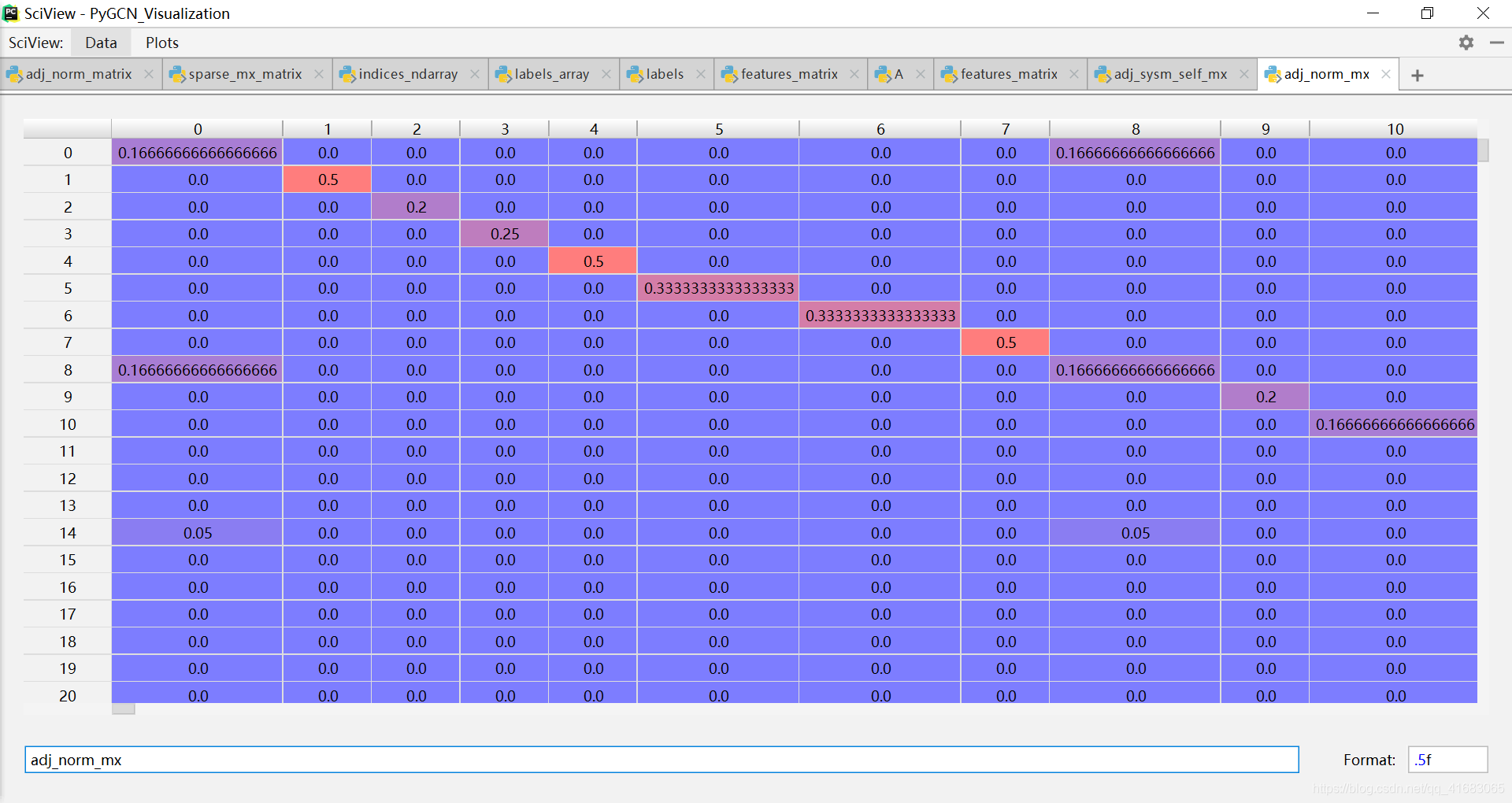
第一行归一化的结果为: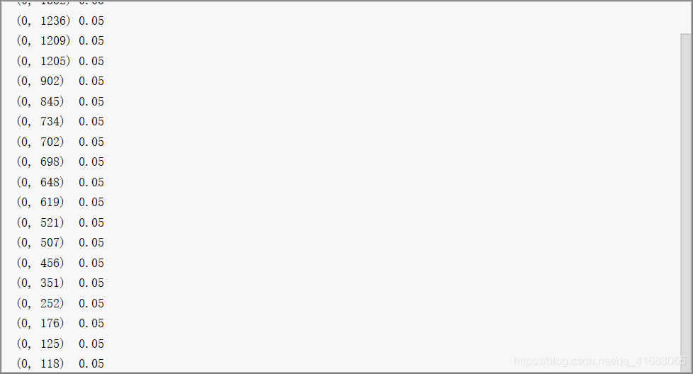
归一化后的值正好是 1 / 20 = 0.05 。
测试该函数的Demo放到下面了:
import numpy as npimport scipy.sparse as spfrom pygcn.utils import normalize'''测试归一化函数'''# 读取原始数据集path="../data/cora/"dataset = "cora"idx_features_labels = np.genfromtxt("{}{}.content".format(path, dataset),dtype=np.dtype(str))RawFeature = idx_features_labels[:, 1:-1]RawFeature=RawFeature.astype(int)sample1_label=RawFeature[0,:]sumA=sample1_label.sum()print("原始的feature\n",RawFeature)# type ndarray# [['0' '0' '0'... '0' '0' '0']# ['0' '0' '0'... '0' '0' '0']# ['0' '0' '0'...'0' '0' '0']# ...# ['0' '0' '0'...'0' '0' '0']# ['0' '0' '0'... '0' '0' '0']# ['0' '0' '0'...'0' '0' '0']]print(RawFeature.shape)# (2708, 1433)features = sp.csr_matrix(idx_features_labels[:, 1:-1], dtype=np.float32)# <2708x1433 sparse matrix of type '<class 'numpy.float32'>'# with 49216 stored elements in Compressed Sparse Row format>print("csr_matrix之后的feature\n",features)# type csr_matrix# (0, 0) 0.0# (0, 1) 0.0# (0, 2) 0.0# (0, 3) 0.0# (0, 4) 0.0# ::# (2707, 1428) 0.0# (2707, 1429) 0.0# (2707, 1430) 0.0# (2707, 1431) 0.0# (2707, 1432) 0.0print(features.shape)# (2708, 1433)# features = normalize(features)rowsum = np.array(features.sum(1)) # (2708, 1)r_inv = np.power(rowsum, -1).flatten() # (2708,)r_inv[np.isinf(r_inv)] = 0. # 处理除数为0导致的infr_mat_inv = sp.diags(r_inv)# <2708x2708 sparse matrix of type '<class 'numpy.float32'>'# with 2708 stored elements (1 diagonals) in DIAgonal format>mx = r_mat_inv.dot(features)print('normalization之后的feature\n',mx)# (0, 176) 0.05# (0, 125) 0.05# (0, 118) 0.05# ::# (1, 1425) 0.05882353# (1, 1389) 0.05882353# (1, 1263) 0.05882353# ::# (2707, 136) 0.05263158# (2707, 67) 0.05263158# (2707, 19) 0.05263158
数据集读取函数:load_data(path, dataset)
'''数据读取'''# 更改路径。由../改为C:\Users\73416\PycharmProjects\PyGCNdef load_data(path="../data/cora/", dataset="cora"):"""Load citation network dataset (cora only for now)"""print('Loading {} dataset...'.format(dataset))'''cora.content 介绍:cora.content共有2708行,每一行代表一个样本点,即一篇论文。每一行由三部分组成:是论文的编号,如31336;论文的词向量,一个有1433位的二进制;论文的类别,如Neural_Networks。总共7种类别(label)第一个是论文编号,最后一个是论文类别,中间是自己的信息(feature)''''''读取feature和label'''# 以字符串形式读取数据集文件:各自的信息。idx_features_labels = np.genfromtxt("{}{}.content".format(path, dataset),dtype=np.dtype(str))# csr_matrix:Compressed Sparse Row marix,稀疏np.array的压缩# idx_features_labels[:, 1:-1]表明跳过论文编号和论文类别,只取自己的信息(feature of node)features = sp.csr_matrix(idx_features_labels[:, 1:-1], dtype=np.float32)# idx_features_labels[:, -1]表示只取最后一个,即论文类别,得到的返回值为int类型的labellabels = encode_onehot(idx_features_labels[:, -1])# build graph# idx_features_labelsidx_features_labels[:, 0]表示取论文编号idx = np.array(idx_features_labels[:, 0], dtype=np.int32)# 通过建立论文序号的序列,得到论文序号的字典idx_map = {j: i for i, j in enumerate(idx)}edges_unordered = np.genfromtxt("{}{}.cites".format(path, dataset),dtype=np.int32)# 进行一次论文序号的映射# 论文编号没有用,需要重新的其进行编号(从0开始),然后对原编号进行替换。# 所以目的是把离散的原始的编号,变成0 - 2707的连续编号edges = np.array(list(map(idx_map.get, edges_unordered.flatten())),dtype=np.int32).reshape(edges_unordered.shape)# coo_matrix():系数矩阵的压缩。分别定义有那些非零元素,以及各个非零元素对应的row和col,最后定义稀疏矩阵的shape。adj = sp.coo_matrix((np.ones(edges.shape[0]), (edges[:, 0], edges[:, 1])),shape=(labels.shape[0], labels.shape[0]),dtype=np.float32)# build symmetric adjacency matrixadj = adj + adj.T.multiply(adj.T > adj) - adj.multiply(adj.T > adj)# feature和adj归一化features = normalize(features)adj = normalize(adj + sp.eye(adj.shape[0]))# train set, validation set, test set的分组。idx_train = range(140)idx_val = range(200, 500)idx_test = range(500, 1500)# 数据类型转tensorfeatures = torch.FloatTensor(np.array(features.todense()))labels = torch.LongTensor(np.where(labels)[1])adj = sparse_mx_to_torch_sparse_tensor(adj)idx_train = torch.LongTensor(idx_train)idx_val = torch.LongTensor(idx_val)idx_test = torch.LongTensor(idx_test)# 返回数据return adj, features, labels, idx_train, idx_val, idx_test
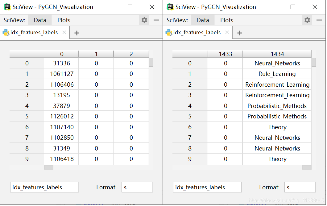
对于Cora数据集来说,读取到的第一手结果是这样的:
- 第一列:各个样本的标号(论文编号)
- 第二列-倒数第二列:各个样本的feature
- 第三列:各个样本的label
labels 预处理
即对 labels 进行 onehot 编码。
# idx_features_labels[:, -1]表示只取最后一个,即论文类别,得到的返回值为int类型的labellabels = encode_onehot(idx_features_labels[:, -1])
feature 预处理
即对 feature 进行归一化。由于 feature 为维度较大的稀疏矩阵,故使用 scipy.sparse 来处理。
# csr_matrix:Compressed Sparse Row marix,稀疏np.array的压缩# idx_features_labels[:, 1:-1]表明跳过论文编号和论文类别,只取自己的信息(feature of node)features = sp.csr_matrix(idx_features_labels[:, 1:-1], dtype=np.float32)……# feature和adj归一化features = normalize(features)
关于处理方法,已经在 特征归一化函数:normalize(mx) 写明了。
构建邻接矩阵 adj
整体来说分两部分:
- 序号预处理:将非连续的离散序号,转化为连续的离散序号(0,1,2,……,2707)。
根据预处理后的序号,将引用关系转化为邻接矩阵adj。
# idx_features_labelsidx_features_labels[:, 0]表示取论文编号idx = np.array(idx_features_labels[:, 0], dtype=np.int32)
这句是从
idx_features_labels中取出idx,即样本的序号(与样本一一对应)# 通过建立论文序号的序列,得到论文序号的字典idx_map = {j: i for i, j in enumerate(idx)}
这句是建立原有的样本序号到连续的离散序号(0,1,2,……,2707)之间的映射关系。
需要说明的是,样本的序号与样本一一对应,即不存在重复的情况,所以排序后的样本序号直接从0开始数就OK。# 读取图的边(论文间的引用关系)# cora.cites共5429行, 每一行有两个论文编号,表示第一个编号的论文先写,第二个编号的论文引用第一个编号的论文。edges_unordered = np.genfromtxt("{}{}.cites".format(path, dataset),dtype=np.int32)
以Cora数据集为例,这一句是从数据集文件中读取论文间的引用关系,即Graph中边。
读取的结果如下所示:[[ 35 1033][ 35 103482][ 35 103515]...[ 853118 1140289][ 853155 853118][ 954315 1155073]]
需要注意,这里的样本序号还是原始的样本序号,还没映射到预处理后的序号。
# 进行一次论文序号的映射# 论文编号没有用,需要重新的其进行编号(从0开始),然后对原编号进行替换。# 所以目的是把离散的原始的编号,变成0 - 2707的连续编号edges = np.array(list(map(idx_map.get, edges_unordered.flatten())),dtype=np.int32).reshape(edges_unordered.shape)
这一句代码实现了样本序号的映射。用到的函数有
map(),list()和reshape()。# coo_matrix():系数矩阵的压缩。分别定义有那些非零元素,以及各个非零元素对应的row和col,最后定义稀疏矩阵的shape。adj = sp.coo_matrix((np.ones(edges.shape[0]), (edges[:, 0], edges[:, 1])),shape=(2708, 2708),dtype=np.float32)
(np.ones(edges.shape[0]):代表稀疏矩阵要填入的值,为1。若邻接矩阵的相应位置被填入1,则说明两个论文中有引用关系。(edges[:, 0], edges[:, 1]):指明了要填入数据的位置,其中edges[:, 0]指明行,edges[:, 1]指明列。shape=(labels.shape[0], labels.shape[0]):指明了adj的shape,为 N × N 的矩阵,其中 N 为样本数。dtype=np.float32:指明了矩阵元素的类型。
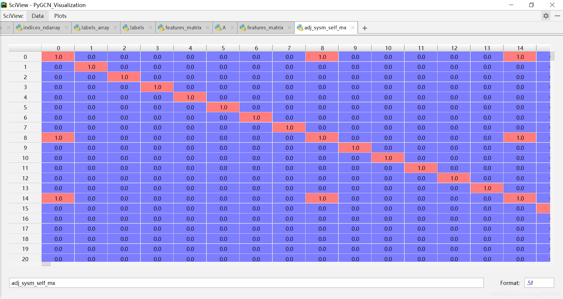
最终adj的类型为:scipy.sparse.coo.coo_matrix,使用np.array(adj.todense)将其转为ndarray类型的稠密矩阵后,如下: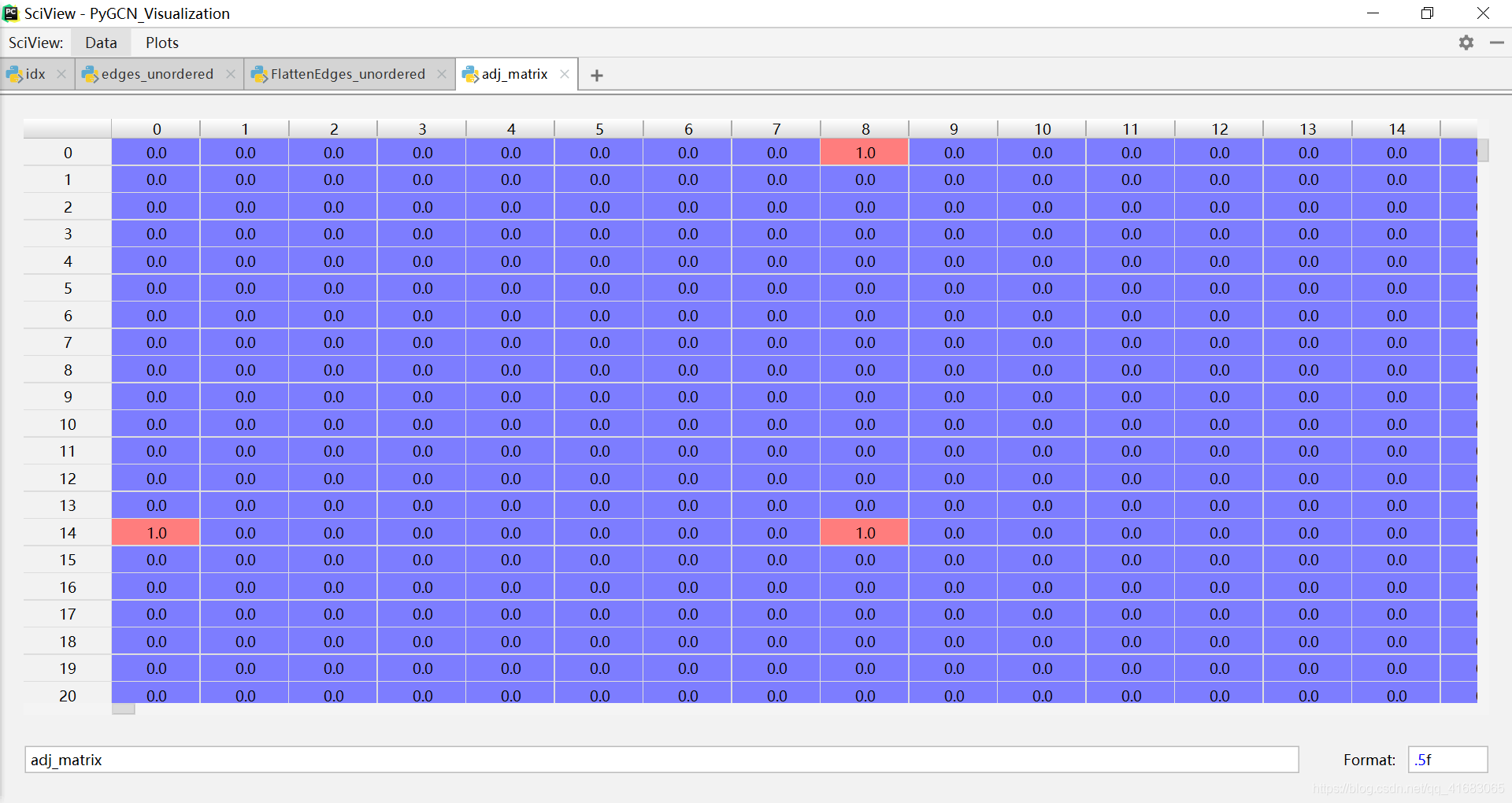
可以看到,由于引用关系的是单向的,导致邻接矩阵adj并不是对称矩阵,构成的Graph也是有向图。
# build symmetric adjacency matrix# np.multiply()函数,数组和矩阵对应位置相乘,输出与相乘数组/矩阵的大小一致adj = adj + adj.T.multiply(adj.T > adj) - adj.multiply(adj.T > adj)
这一步是将非对称的邻接矩阵adj,变为对称矩阵。表现在图上,结果就是将有向图变为无向图。
得到的邻接矩阵 adj 如下(可与上面的对比)(如果要使用有向图的邻接矩阵,把这一句注释掉就行):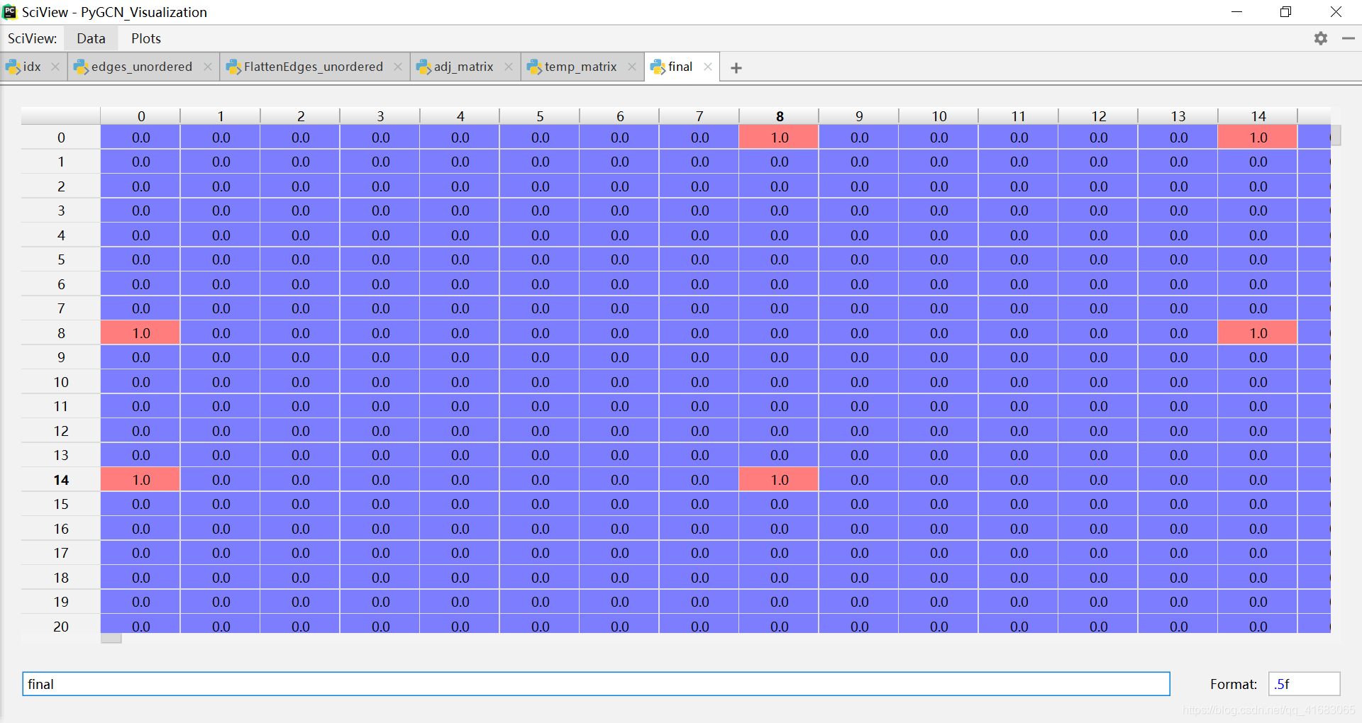
adj = normalize(adj + sp.eye(adj.shape[0])) # adj在归一化之前,先引入自环
数据集划分
# train set, validation set, test set的分组。idx_train = range(140)idx_val = range(200, 500)idx_test = range(500, 1500)
按照序号划分数据集。这种划分方式并不是论文中的划分方法。论文中是每一类取相同个数 n个样本作为训练集。
数据类型转为tensor
# 数据类型转tensorfeatures = torch.FloatTensor(np.array(features.todense()))labels = torch.LongTensor(np.where(labels)[1])adj = sparse_mx_to_torch_sparse_tensor(adj)idx_train = torch.LongTensor(idx_train)idx_val = torch.LongTensor(idx_val)idx_test = torch.LongTensor(idx_test)
adj:对于邻接矩阵adj的操作,sparse_mx_to_torch_sparse_tensor(adj),是 Convert a scipy sparse matrix to a torch sparse tensor。具体的细节请看:稀疏矩阵转稀疏张量函数:sparse_mx_to_torch_sparse_tensor(sparse_mx)labels:有一点很有意思,是labels的返回值,这个返回值是长这样的:
这就很奇怪。也就是说返回的标签labels还是int类型的,而不是onehot编码后的结果。这样看来onehot编码并没有起到作用,因为我直接将标签映射到int就可以,而不必须要经过onehot编码这个中间步骤。
在主函数验证,load_data()函数的返回值labels信息如下:
tensor([4, 2, 0, ..., 1, 6, 4])<class 'torch.Tensor'>torch.Size([2708])
跟上图显示的一致,即load_data()的返回值labels并不是onehot编码的结果,而是0,1,……,6这样的标签。features:是转成了正常的tensor类型(不是adj那样的类型):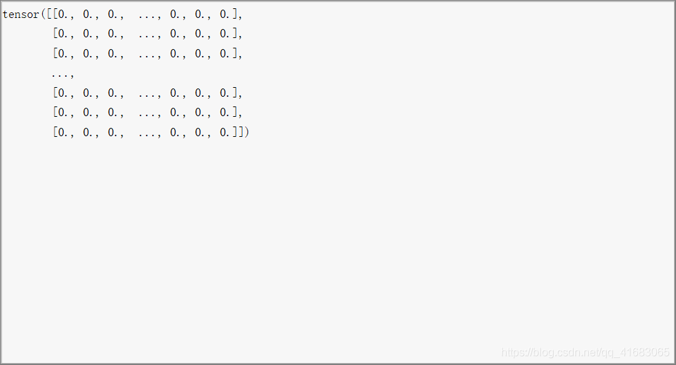
返回数据
# 返回数据return adj, features, labels, idx_train, idx_val, idx_test
整个debug load_data()的Demo放到下面了,想尝试的可以拿去用:
import numpy as npimport scipy.sparse as spfrom pygcn.utils import normalize,sparse_mx_to_torch_sparse_tensor,encode_onehotimport torch'''测试论文编号处理'''# 读取原始数据集path="C:/Users/73416/PycharmProjects/PyGCN_Visualization/data/cora/"dataset = "cora"idx_features_labels = np.genfromtxt("{}{}.content".format(path, dataset),dtype=np.dtype(str))# build graph# idx_features_labelsidx_features_labels[:, 0]表示取论文编号idx = np.array(idx_features_labels[:, 0], dtype=np.int32)# 通过建立论文序号的序列,得到论文序号的字典idx_map = {j: i for i, j in enumerate(idx)}# 读取图的边(论文间的引用关系)# cora.cites共5429行, 每一行有两个论文编号,表示第一个编号的论文先写,第二个编号的论文引用第一个编号的论文。edges_unordered = np.genfromtxt("{}{}.cites".format(path, dataset),dtype=np.int32)# 进行一次论文序号的映射# 论文编号没有用,需要重新的其进行编号(从0开始),然后对原编号进行替换。# 所以目的是把离散的原始的编号,变成0 - 2707的连续编号edges = np.array(list(map(idx_map.get, edges_unordered.flatten())),dtype=np.int32).reshape(edges_unordered.shape)# coo_matrix():系数矩阵的压缩。分别定义有那些非零元素,以及各个非零元素对应的row和col,最后定义稀疏矩阵的shape。adj = sp.coo_matrix((np.ones(edges.shape[0]), (edges[:, 0], edges[:, 1])),shape=(2708, 2708),dtype=np.float32)# build symmetric adjacency matrixadj_sysm = adj + adj.T.multiply(adj.T > adj) - adj.multiply(adj.T > adj)# 引入自环adj_sysm_self= adj_sysm + sp.eye(adj.shape[0])# 归一化adj_norm = normalize(adj_sysm_self)features = sp.csr_matrix(idx_features_labels[:, 1:-1], dtype=np.float32)features = normalize(features)labels = encode_onehot(idx_features_labels[:, -1])# 数据类型转tensorfeatures = torch.FloatTensor(np.array(features.todense()))labels = torch.LongTensor(np.where(labels)[1])adj_norm = sparse_mx_to_torch_sparse_tensor(adj_norm)# 测试sparse_mx_to_torch_sparse_tensor(sparse_mx)函数# sparse_mx = adj_norm.tocoo().astype(np.float32)# indices = torch.from_numpy(# np.vstack((sparse_mx.row, sparse_mx.col)).astype(np.int64))# values = torch.from_numpy(sparse_mx.data)# shape = torch.Size(sparse_mx.shape)# 增加于2020.3.12,返回非对称邻接矩阵,构成有向图adj_directed_self=adj+ sp.eye(adj.shape[0])adj_directed_self_matrix=np.array(adj_directed_self.todense())adj_directed_norm=normalize(adj_directed_self)adj_directed_norm_matrix=np.array(adj_directed_norm.todense())
计算准确率函数:accuracy(output, labels)
'''计算accuracy'''def accuracy(output, labels):preds = output.max(1)[1].type_as(labels)correct = preds.eq(labels).double()correct = correct.sum()return correct / len(labels)
输出和输入:
output为模型model直接的输出,并不是单个的标签(获取预测类别的操作在accuracy(output, labels))中的preds = output.max(1)[1].type_as(labels)实现)。其信息为:tensor([[-5.3865, -5.8370, -5.6641, ..., -0.0546, -4.6866, -5.4952],[-1.9110, -3.6502, -0.8442, ..., -3.3036, -1.5383, -2.0366],[-0.1619, -3.4708, -3.5892, ..., -3.9754, -3.4787, -3.3948],...,[-1.9098, -0.5042, -3.1999, ..., -3.0369, -3.6273, -2.5525],[-2.6523, -2.9252, -2.6154, ..., -3.0894, -3.3290, -0.3564],[-4.6700, -4.5324, -4.5864, ..., -0.0916, -4.3737, -3.9876]],device='cuda:0', grad_fn=<LogSoftmaxBackward>)<class 'torch.Tensor'>torch.Size([2708, 7])
labels的传入形式:[4 2 0 ... 1 6 4]<class 'numpy.ndarray'>(2708,)
稀疏矩阵转稀疏张量函数:sparse_mx_to_torch_sparse_tensor(sparse_mx)
'''稀疏矩阵转稀疏张量'''def sparse_mx_to_torch_sparse_tensor(sparse_mx):"""Convert a scipy sparse matrix to a torch sparse tensor."""sparse_mx = sparse_mx.tocoo().astype(np.float32)indices = torch.from_numpy(np.vstack((sparse_mx.row, sparse_mx.col)).astype(np.int64))values = torch.from_numpy(sparse_mx.data)shape = torch.Size(sparse_mx.shape)return torch.sparse.FloatTensor(indices, values, shape)
其中,传入函数的
sparse_mx是长这样的:
sparse_mx = sparse_mx.tocoo().astype(np.float32)之后的sparse_mx是长这样的:

也就是说,矩阵还是那个矩阵,只不过通过.tocoo()将矩阵的形式变成了COOrdinate format。
csr_matrix.tocoo(*self*, *copy=True*)Convert this matrix to COOrdinate format.With copy=False, the data/indices may be shared between this matrix and the resultant coo_matrix.
indices = torch.from_numpy(np.vstack((sparse_mx.row, sparse_mx.col)).astype(np.int64))这一句是提取稀疏矩阵的非零元素的索引。得到的矩阵是一个[2, 8137]的tensor。
其中第一行是行索引,第二行是列索引。每一列的两个值对应一个非零元素的坐标。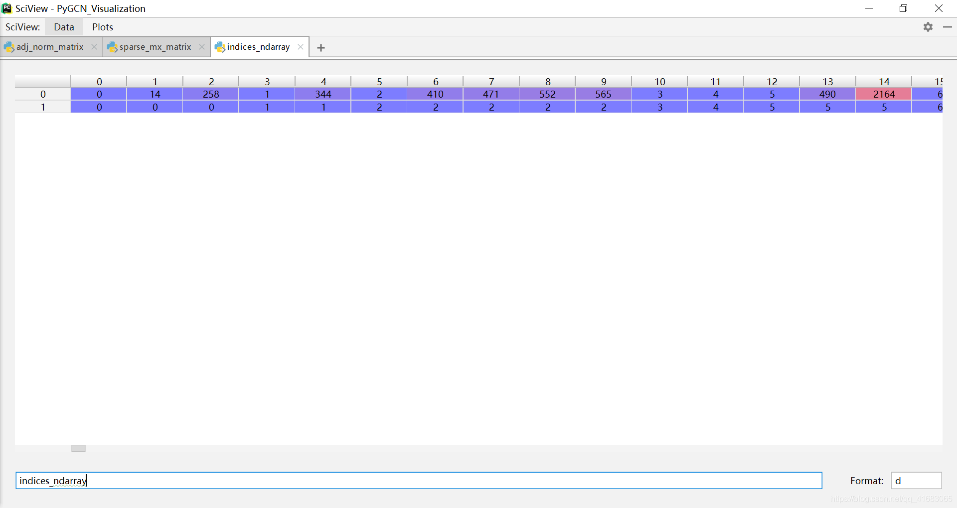
values = torch.from_numpy(sparse_mx.data)、shape = torch.Size(sparse_mx.shape) 这两行就是规定了数值和shape。没什么好说的。
return torch.sparse.FloatTensor(indices, values, shape)
函数返回值应该注意一下。该函数的返回值的类型是 torch.Tensor。
直接打印的结果是一个对象:
print(torch.Tensor)<class 'torch.Tensor'>
具体查看的话是这样: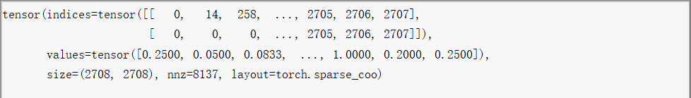
说明返回的是一个类的实例!torch.sparse的官方文档如下:
Torch supports sparse tensors in COO(rdinate) format, which can efficiently store and process tensors for which the majority of elements are zeros.A sparse tensor is represented as a pair of dense tensors: a tensor of values and a 2D tensor of indices. A sparse tensor can be constructed by providing these two tensors, as well as the size of the sparse tensor (which cannot be inferred from these tensors!)
layers.py
全部源代码放到前面:
import mathimport torchfrom torch.nn.parameter import Parameterfrom torch.nn.modules.module import Moduleclass GraphConvolution(Module):"""Simple GCN layer, similar to https://arxiv.org/abs/1609.02907"""'''定义对象的属性'''def __init__(self, in_features, out_features, bias=True):super(GraphConvolution, self).__init__()self.in_features = in_featuresself.out_features = out_featuresself.weight = Parameter(torch.FloatTensor(in_features, out_features)) # in_features × out_featuresif bias:self.bias = Parameter(torch.FloatTensor(out_features))else:self.register_parameter('bias', None)self.reset_parameters()'''生成权重'''def reset_parameters(self):stdv = 1. / math.sqrt(self.weight.size(1))self.weight.data.uniform_(-stdv, stdv) # .uniform():将tensor用从均匀分布中抽样得到的值填充。if self.bias is not None:self.bias.data.uniform_(-stdv, stdv)'''前向传播 of 一层之内:即本层的计算方法:A_hat * X * W '''def forward(self, input, adj):support = torch.mm(input, self.weight) # torch.mm:Matrix multiply,input和weight实现矩阵点乘。output = torch.spmm(adj, support) # torch.spmm:稀疏矩阵乘法,sp即sparse。if self.bias is not None:return output + self.biaselse:return output'''把一个对象用字符串的形式表达出来以便辨认,在终端调用的时候会显示信息'''def __repr__(self):return self.__class__.__name__ + ' (' \+ str(self.in_features) + ' -> ' \+ str(self.out_features) + ')'
GraphConvolution是图数据实现卷积操作的层,类似于CNN中的卷积层,只是一个层而已。GraphConvolution作为一个类,首先要定义其属性:
'''定义对象的属性'''def __init__(self, in_features, out_features, bias=True):super(GraphConvolution, self).__init__()self.in_features = in_featuresself.out_features = out_featuresself.weight = Parameter(torch.FloatTensor(in_features, out_features)) # in_features × out_featuresif bias:self.bias = Parameter(torch.FloatTensor(out_features))else:self.register_parameter('bias', None)self.reset_parameters()
主要包括两部分:
- 设定该层中
in_features和out_features - 参数的初始化,通过该对象的
reset_parameters()方法实现。参数包括:weight:维度为in_features×out_featuresbias( if True ):维度为out_features```python ‘’’生成权重’’’ def resetparameters(self): stdv = 1. / math.sqrt(self.weight.size(1)) self.weight.data.uniform(-stdv, stdv) # .uniform():将tensor用从均匀分布中抽样得到的值填充。 if self.bias is not None: self.bias.data.uniform_(-stdv, stdv)
就是随机生成权重,不细说了。<br />但是有一点,生成随机数的种子是可以认为设定的([设定随机数种子](https://blog.csdn.net/qq_41683065/article/details/104627989?utm_medium=distribute.pc_relevant.none-task-blog-BlogCommendFromMachineLearnPai2-1.compare&depth_1-utm_source=distribute.pc_relevant.none-task-blog-BlogCommendFromMachineLearnPai2-1.compare#%E8%AE%BE%E5%AE%9A%E9%9A%8F%E6%9C%BA%E6%95%B0%E7%A7%8D%E5%AD%90)),即可以每次初始化得到相同的初始化参数,从而使得结果可复现。```python'''前向传播 of 一层之内:即本层的计算方法:A * X * W '''def forward(self, input, adj):support = torch.mm(input, self.weight) # torch.mm:Matrix multiply,input和weight实现矩阵点乘。output = torch.spmm(adj, support) # torch.spmm:稀疏矩阵乘法,sp即sparse。if self.bias is not None:return output + self.biaselse:return output
这一层是定义的本层的前向传播,即本层的计算方法:A ∗ X ∗ W support = torch.mm(input, self.weight)是input和weight实现矩阵乘法,即support = X ∗ W。output = torch.spmm(adj, support),由于adj是torch.sparse的对象,所以要使用稀疏矩阵乘法torch.spmm(),实现的功能是得到outpuy=A∗support。
然后再加上bias ( if True ),就得到了本层最后的输出。
'''把一个对象用字符串的形式表达出来以便辨认,在终端调用的时候会显示信息'''def __repr__(self):return self.__class__.__name__ + ' (' \+ str(self.in_features) + ' -> ' \+ str(self.out_features) + ')'
models.py
全部源代码放到前面:
import torch.nn as nnimport torch.nn.functional as Ffrom pygcn.layers import GraphConvolution'''GCN类'''class GCN(nn.Module):def __init__(self, nfeat, nhid, nclass, dropout):super(GCN, self).__init__()self.gc1 = GraphConvolution(nfeat, nhid) # 第一层self.gc2 = GraphConvolution(nhid, nclass) # 第二层self.dropout = dropout # 定义dropout'''前向传播 of 层间:整个网络的前向传播的方式:relu(gc1) --> dropout --> gc2 --> log_softmax'''def forward(self, x, adj):x = F.relu(self.gc1(x, adj))x = F.dropout(x, self.dropout, training=self.training)x = self.gc2(x, adj)return F.log_softmax(x, dim=1)
class GCN(nn.Module)定义了一个图卷积神经网络,在这里有两个卷积层。
该对象的属性为:
def __init__(self, nfeat, nhid, nclass, dropout):super(GCN, self).__init__()self.gc1 = GraphConvolution(nfeat, nhid) # 第一层self.gc2 = GraphConvolution(nhid, nclass) # 第二层self.dropout = dropout
gc1:in_feature= nfeat,为数据的原始的feature。out_feature= nhid。gc2:in_feature= nhid。out_feature= nclass,为最后待分类的类别数。dropout
整个网络的前向传播为:
'''前向传播 of 层间:整个网络的前向传播的方式:relu(gc1) --> dropout --> gc2 --> log_softmax'''def forward(self, x, adj):x = F.relu(self.gc1(x, adj))x = F.dropout(x, self.dropout, training=self.training)x = self.gc2(x, adj)return F.log_softmax(x, dim=1)
整个网络的前向传播:整个网络的前向传播的方式:relu(gc1) —> dropout —> gc2 —> log_softmax
train.py
from __future__ import divisionfrom __future__ import print_functionimport timeimport argparseimport numpy as npimport torchimport torch.nn.functional as Fimport torch.optim as optimfrom utils import load_data, load_data2, accuracyfrom models import GCN# Training settingsparser = argparse.ArgumentParser()parser.add_argument('--no-cuda', action='store_true', default=False,help='Disables CUDA training.')parser.add_argument('--fastmode', action='store_true', default=False,help='Validate during training pass.')parser.add_argument('--seed', type=int, default=42, help='Random seed.')parser.add_argument('--epochs', type=int, default=100,help='Number of epochs to train.')parser.add_argument('--lr', type=float, default=0.01,help='Initial learning rate.')parser.add_argument('--weight_decay', type=float, default=5e-4,help='Weight decay (L2 loss on parameters).')parser.add_argument('--hidden', type=int, default=16,help='Number of hidden units.')parser.add_argument('--dropout', type=float, default=0.5,help='Dropout rate (1 - keep probability).')args = parser.parse_args()args.cuda = not args.no_cuda and torch.cuda.is_available()#作为是否使用cpu的判定#设计随机数种子np.random.seed(args.seed)torch.manual_seed(args.seed)if args.cuda:torch.cuda.manual_seed(args.seed)# Load dataadj, features, labels, idx_train, idx_val, idx_test = load_data()#adj, features, labels, idx_train, idx_val, idx_test = load_data2("BlogCatalog")# Model and optimizer# Modelmodel = GCN(nfeat=features.shape[1],nhid=args.hidden,nclass=labels.max().item() + 1, # 对Cora数据集,为7,即类别总数。dropout=args.dropout)optimizer = optim.Adam(model.parameters(),lr=args.lr, weight_decay=args.weight_decay)if args.cuda:model.cuda()features = features.cuda()adj = adj.cuda()labels = labels.cuda()idx_train = idx_train.cuda()idx_val = idx_val.cuda()idx_test = idx_test.cuda()def train(epoch):t = time.time()'''将模型转为训练模式,并将优化器梯度置零'''model.train()optimizer.zero_grad()'''计算输出时,对所有的节点计算输出'''output = model(features, adj)'''损失函数,仅对训练集节点计算,即:优化仅对训练集数据进行'''loss_train = F.nll_loss(output[idx_train], labels[idx_train])# 计算准确率acc_train = accuracy(output[idx_train], labels[idx_train])# 反向传播loss_train.backward()# 优化optimizer.step()'''fastmode ? '''if not args.fastmode:# Evaluate validation set performance separately,# deactivates dropout during validation run.model.eval()output = model(features, adj)'''验证集 loss 和 accuracy '''loss_val = F.nll_loss(output[idx_val], labels[idx_val])acc_val = accuracy(output[idx_val], labels[idx_val])'''输出训练集+验证集的 loss 和 accuracy '''print('Epoch: {:04d}'.format(epoch+1),'loss_train: {:.4f}'.format(loss_train.item()),'acc_train: {:.4f}'.format(acc_train.item()),'loss_val: {:.4f}'.format(loss_val.item()),'acc_val: {:.4f}'.format(acc_val.item()),'time: {:.4f}s'.format(time.time() - t))def test():model.eval() # model转为测试模式output = model(features, adj)loss_test = F.nll_loss(output[idx_test], labels[idx_test])acc_test = accuracy(output[idx_test], labels[idx_test])print("Test set results:","loss= {:.4f}".format(loss_test.item()),"accuracy= {:.4f}".format(acc_test.item()))# return output # 可视化返回output# Train modelt_total = time.time()for epoch in range(args.epochs):train(epoch)print("Optimization Finished!")print("Total time elapsed: {:.4f}s".format(time.time() - t_total))# Testingtest()
调用所需要的函数库
from __future__ import divisionfrom __future__ import print_functionimport timeimport argparseimport numpy as npimport torchimport torch.nn.functional as Fimport torch.optim as optimfrom utils import load_data, load_data2, accuracyfrom models import GCN
版本兼容
from __future__ import divisionfrom __future__ import print_function
- 第一条语句:
在 Python2 中导入未来的支持的语言特征中division (精确除法),即from __future__ import division,当我们在程序中没有导入该特征时,”/“操作符执行的只能是整除,也就是取整数,只有当我们导入division(精确算法)以后,”/“执行的才是精确算法。 - 第二条语句:
在开头加上from __future__ import print_function这句之后,即使在python2.X,使用print就得像python3.X那样加括号使用。python2.X中print不需要括号,而在python3.X中则需要。argparse是一个Python模块:命令行选项、参数和子命令解析器
```pythonTraining settings
parser = argparse.ArgumentParser() parser.add_argument(‘—no-cuda’, action=’store_true’, default=False,
parser.add_argument(‘—fastmode’, action=’store_true’, default=False,help='Disables CUDA training.')
parser.add_argument(‘—seed’, type=int, default=42, help=’Random seed.’) parser.add_argument(‘—epochs’, type=int, default=100,help='Validate during training pass.')
parser.add_argument(‘—lr’, type=float, default=0.01,help='Number of epochs to train.')
parser.add_argument(‘—weight_decay’, type=float, default=5e-4,help='Initial learning rate.')
parser.add_argument(‘—hidden’, type=int, default=16,help='Weight decay (L2 loss on parameters).')
parser.add_argument(‘—dropout’, type=float, default=0.5,help='Number of hidden units.')
help='Dropout rate (1 - keep probability).')
args = parser.parse_args()#生成超参数 args.cuda = not args.no_cuda and torch.cuda.is_available()#作为是否使用cpu的判定
[Python- argparse.ArgumentParser()用法解析](https://blog.csdn.net/huima2017/article/details/104797135)<br />[parse_args(argsparse):python和命令行之间的交互](https://www.cnblogs.com/still-smile/p/11636958.html)<a name="QdVYW"></a>## 设计随机数种子```python#设计随机数种子np.random.seed(args.seed)torch.manual_seed(args.seed)if args.cuda:torch.cuda.manual_seed(args.seed)
np.random.seed()函数是为CPU运行设定种子,使得CPU运行时产生的随机数一样。比如下面的示例:
# 随机数一样random.seed(1)print('随机数3:',random.random())random.seed(1)print('随机数4:',random.random())random.seed(2)print('随机数5:',random.random())'''随机数1: 0.7643602170615428随机数2: 0.31630323818329664随机数3: 0.13436424411240122随机数4: 0.13436424411240122随机数5: 0.9560342718892494'''
torch.manual_seed()函数是为GPU运行设定种子,使得GPU运行时产生的随机数一样。
比如下面的 Demo:
torch.manual_seed(2) #为CPU设置种子用于生成随机数,以使得结果是确定的print(torch.rand(2))if args.cuda:torch.cuda.manual_seed(args.seed) #为当前GPU设置随机种子;# 如果使用多个GPU,应该使用 torch.cuda.manual_seed_all()为所有的GPU设置种子。
通过设定随机数种子的好处是,使模型初始化的可学习参数相同,从而使每次的运行结果可以复现。
读取数据
# Load dataadj, features, labels, idx_train, idx_val, idx_test = load_data()
读取的结果都是tensor类型的。其中各个变量:
adj:是torch.sparse,已进行归一化features:归一化后的特征labels:int类型的标签,注意并不是onehot编码的形式。具体如下:tensor([4, 2, 0, ..., 1, 6, 4])<class 'torch.Tensor'>torch.Size([2708])
idx_train、idx_val、idx_test:训练集、验证集、测试集中样本的序号。定义模型
# Modelmodel = GCN(nfeat=features.shape[1],nhid=args.hidden,nclass=labels.max().item() + 1, # 对Cora数据集,为7,即类别总数。dropout=args.dropout)
主要是设定
nfeat、nhid、nclass和dropout这四个参数值。定义优化器
# optimizeroptimizer = optim.Adam(model.parameters(),lr=args.lr, weight_decay=args.weight_decay)
选用Adam优化函数,学习率
lr,weight_dacay由命令行指定。CPU转CUDA
# to CUDAif args.cuda:model.cuda()features = features.cuda()adj = adj.cuda()labels = labels.cuda()idx_train = idx_train.cuda()idx_val = idx_val.cuda()idx_test = idx_test.cuda()
训练函数:train(epoch)
def train(epoch):t = time.time()'''将模型转为训练模式,并将优化器梯度置零'''model.train()optimizer.zero_grad()'''计算输出时,对所有的节点计算输出'''output = model(features, adj)'''损失函数,仅对训练集节点计算,即:优化仅对训练集数据进行'''loss_train = F.nll_loss(output[idx_train], labels[idx_train])# 计算准确率acc_train = accuracy(output[idx_train], labels[idx_train])# 反向传播loss_train.backward()# 优化optimizer.step()'''fastmode ? '''if not args.fastmode:# Evaluate validation set performance separately,# deactivates dropout during validation run.model.eval()output = model(features, adj)'''验证集 loss 和 accuracy '''loss_val = F.nll_loss(output[idx_val], labels[idx_val])acc_val = accuracy(output[idx_val], labels[idx_val])'''输出训练集+验证集的 loss 和 accuracy '''print('Epoch: {:04d}'.format(epoch+1),'loss_train: {:.4f}'.format(loss_train.item()),'acc_train: {:.4f}'.format(acc_train.item()),'loss_val: {:.4f}'.format(loss_val.item()),'acc_val: {:.4f}'.format(acc_val.item()),'time: {:.4f}s'.format(time.time() - t))
传入参数
epoch为:当前训练的epoch数。
训练函数在循环中被调用,train()函数本身没有循环(即train()函数表示一次循环的步骤)。训练初始化
'''将模型转为训练模式,并将优化器梯度置零'''model.train()optimizer.zero_grad()
计算模型输出结果
'''计算输出时,对所有的节点计算输出'''output = model(features, adj)
计算model输出,总是对全部样本进行。在计算损失和反向传播时,才对训练集、验证集、测试集进行分别的操作。
计算训练集损失
'''损失函数,仅对训练集节点计算,即:优化仅对训练集数据进行'''loss_train = F.nll_loss(output[idx_train], labels[idx_train])# 计算准确率acc_train = accuracy(output[idx_train], labels[idx_train])
半监督的代码实现,是仅仅对训练集(即:我们认为标签已知的子集)计算损失函数。
反向传播及优化
# 反向传播loss_train.backward()# 优化optimizer.step()
反向传播对训练集数据进行(即:我们认为标签已知的子集)。
通过计算训练集损失和反向传播及优化,带标签的 label 信息就可以 smooth 到整个图上(label information is smoothed over the graph)。计算验证集结果
'''验证集 loss 和 accuracy '''loss_val = F.nll_loss(output[idx_val], labels[idx_val])acc_val = accuracy(output[idx_val], labels[idx_val])
打印训练集和验证集的结果信息
'''输出训练集+验证集的 loss 和 accuracy '''print('Epoch: {:04d}'.format(epoch+1),'loss_train: {:.4f}'.format(loss_train.item()),'acc_train: {:.4f}'.format(acc_train.item()),'loss_val: {:.4f}'.format(loss_val.item()),'acc_val: {:.4f}'.format(acc_val.item()),'time: {:.4f}s'.format(time.time() - t))
测试函数:test()
def test():model.eval() # model转为测试模式output = model(features, adj)loss_test = F.nll_loss(output[idx_test], labels[idx_test])acc_test = accuracy(output[idx_test], labels[idx_test])print("Test set results:","loss= {:.4f}".format(loss_test.item()),"accuracy= {:.4f}".format(acc_test.item()))
先是通过
model.eval()转为测试模式,之后计算输出,并单独对测试集计算损失函数和准确率。训练模型
# Train modelt_total = time.time()for epoch in range(args.epochs):train(epoch)print("Optimization Finished!")print("Total time elapsed: {:.4f}s".format(time.time() - t_total))
调用
epochs次循环,其中 train(epoch) 是一次训练。测试模型
# Testingtest()
数据集cara

若有收获,就点个赞吧
0 人点赞
