[第一部分]神经网络

sigmoid

所谓激活函数,其实就是我们将某些数值定义为某种语义…比如在sigmoid激活函数中,我们把数值的大小定义为可能性的高低, 数值越小我们定义越为不可能, 数值越大我们定义为越可能….所以, 发现了吗?

1. 通过激活函数,我们将冰冷的数值表达为了我们更方便理解的语义信息.
2. 至于为什么sigmoid函数的公式是这样的吗? 无非这种公式在将冰冷数值表达为语义信息方面做得更好.

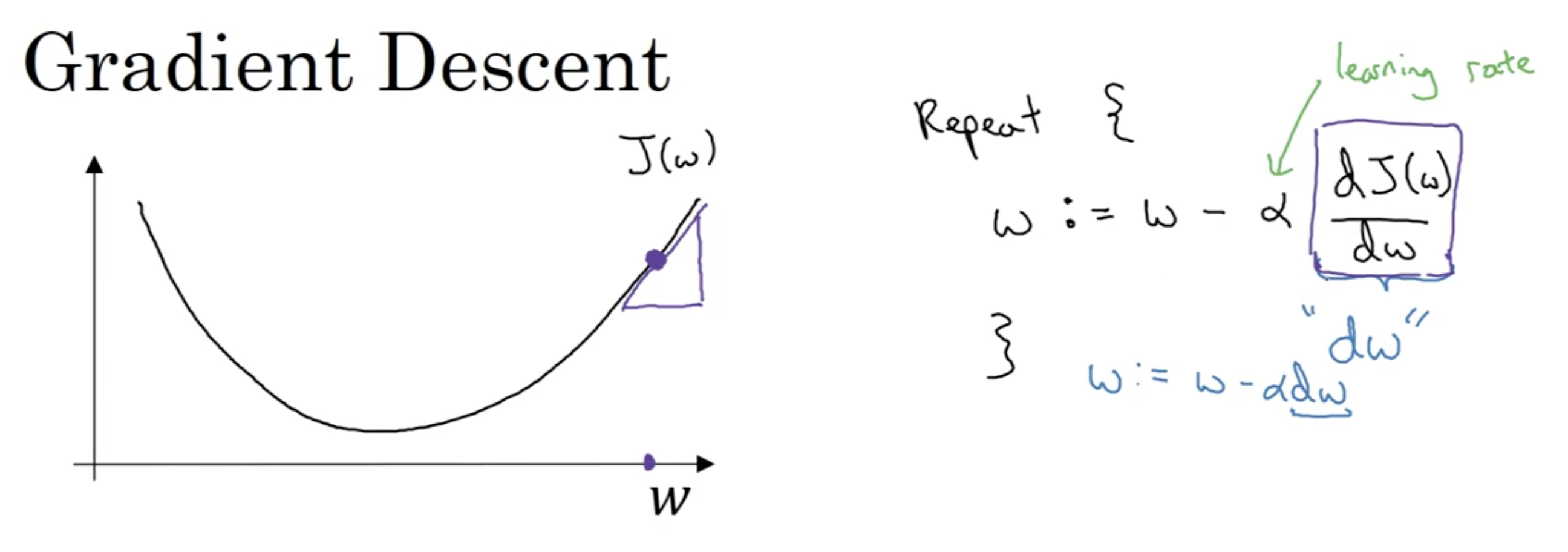
代价(损失)函数与梯度下降

如上是逻辑回归的损失函数在进行梯度下降来找到更好的模型参数…

为什么需要损失函数呢? 这是因为在前面的激活函数中,我们已经能够将冰冷的数值表达我更容易理解的语义信息, 但是仍然有个问题, 模型虽然给出了语义, 但它给出的语义并不是正确的呀 ? 所以呢: 这时候就需要机器学习起来了,让它输出的语义信息变得更准确, 甚至希望准确到, 让我们可以无条件相信它给出的答案… 但是, 怎么做呢? 于是就出现了损失函数, 损失函数的目的就是去表达模型的好坏(尽管, 这种评价可能并不完全正确), 换句话说:

1. 我们让损失函数的高低与模型的每一个可学习的参数都是有联系的, 于是乎, 我们只需要通过某种方式(比如梯度下降)让损失函数变得低, 以调整模型参数, 进而让模型变得更好.
2. 但是, 你逻辑回归的损失函数为什么是这样的公式吗? 第一, 该公式的确能比较好地表达模型的好坏; 第二, 该函数是“凹函数”, 在进行梯度下降时, 能更容易更快地收敛到或接近全局最优点.(注: 该特性, 也让逻辑回归的损失函数几乎适用所有初始化方式)
3. 综上: 损失函数的设计尤为关键, 因为, 在训练模型的过程中, 我们不仅要依靠损失函数来表达模型的好坏, 而且还要让损失函数自身更容易收敛到全局最优点. 另外, 有时会对损失函数采用取对数等方式, 可能与加快计算或极大似然估计等有关.

计算图与梯度下降

如上的计算图…

首先, 梯度是什么意思呢? 梯度下降又是什么意思呢? 梯度又是怎么得到的呢?

1. 梯度的定义(最大方向导数): 一个向量，表示某一函数在该点处的方向导数沿着该方向取得最大值，即函数在该点处沿着该方向（此梯度的方向）变化最快，变化率最大. 注意梯度与偏导数的公式联系, 见下:
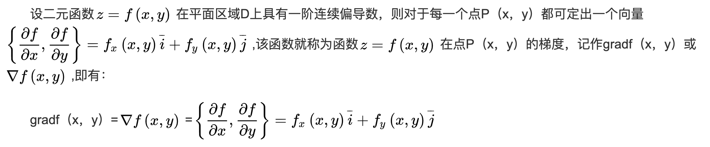
2. 梯度下降: 顾名思义, 就是沿着梯度的方向, 以最快地下降到损失函数的底部. (为什么要到达损失函数的底部在前面已经说过了)
3. 梯度计算: 根据微积分的链式求导法则, 我们能知道在每个参数在损失函数的当前点的一阶偏导数, 由这些参数的一阶偏导数构成的向量即是梯度.
4. 怎么实现损失函数的梯度下降呢? 其实并不是直接用梯度去更新所有参数, 而是在损失函数构成的空间中, 每个参数都在该空间中的一个维度上, 我们只要让每一个参数都”沿着自身维度的方向和其一阶偏导数”(注: 可理解为该参数相对于自身的梯度)(以及学习率)去更新自身,全部的这些改变, 最终体现出来就是损失函数变小了.
5. 如下, m个样本时的梯度下降(左右各为遍历版本和向量化的版本):

numpy向量的一点说明

如上所示, don’t use “rank 1 array”, 其既不是行向量, 也不是列向量. 所以为了避免不必要麻烦, 我们尽量使用列或行向量形式. 另外, 日常使用断言,能有效避免尺寸不匹配问题.

逻辑回归损失函数的数学解释…

图1: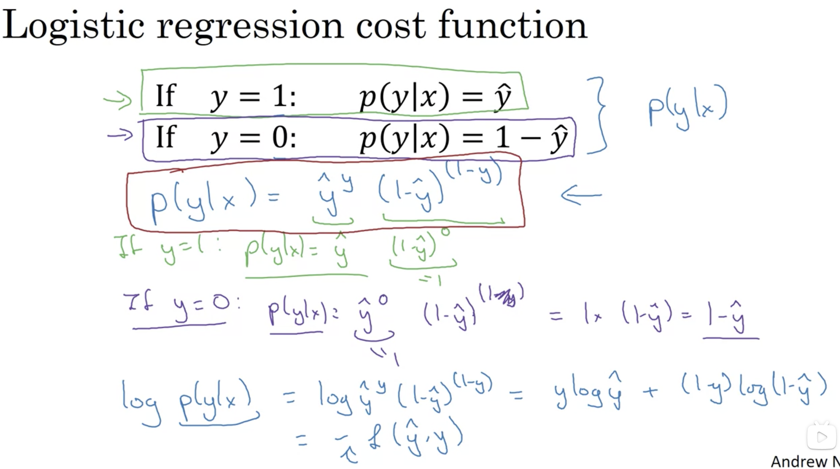

由图1, 可知到逻辑回归的损失函数L被定义为logp(y|x), 而p(y|x)又可等价表示为上图中的数学公式 , 该定义会在图2中用到.

图: 2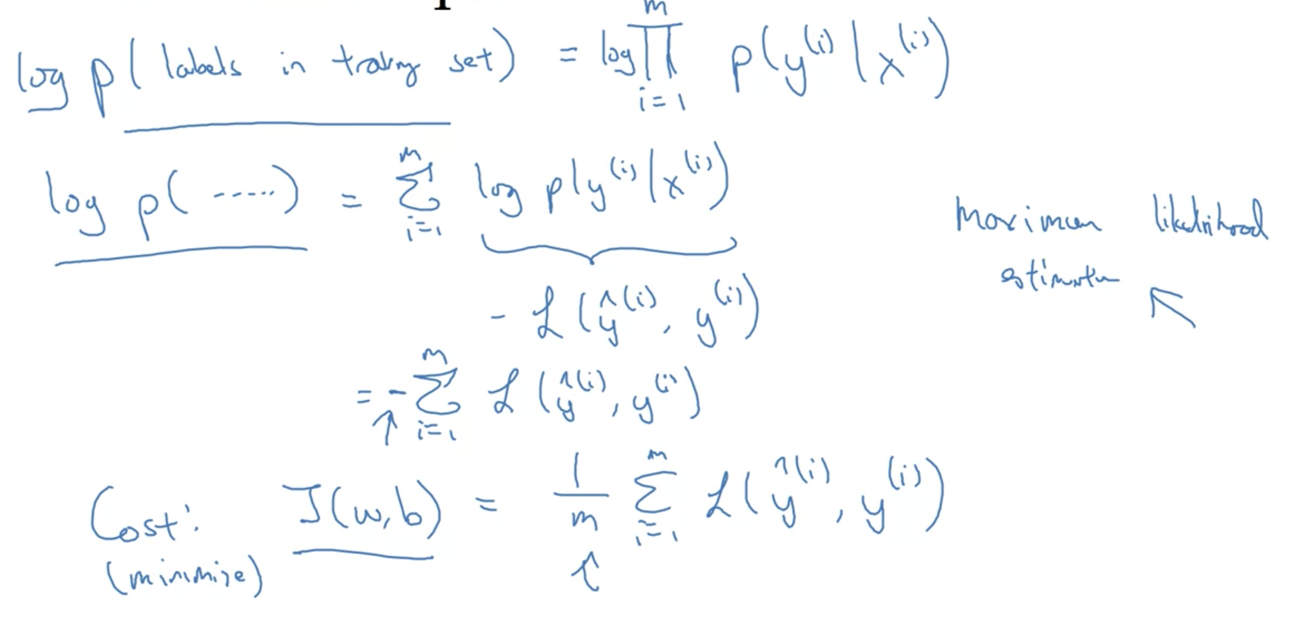

如上,以m个样本的逻辑回归的损失函数为例

首先, 基本的数学原理是极大似然估计, 在逻辑回归的损失函数中, 具体是负对数极大似然估计. (注: 极大似然估计方法（Maximum Likelihood Estimate，MLE）也称为最大概似估计或最大似然估计，是求估计的另一种方法.我们通过已经给定的样本x1~xn(独立同分布)来估计参数, 该估计的前提背景是我们认为现有的样本当前分布中最常见的样本)
如下是似然函数的定义:

在当前背景下, 对数似然函数为下式, 其目的是根据样本x们来估计参数y们, 本质的估计方法为极大似然估计.

在极大化似然函数时, 对其两边取对数不仅能简化运算, 而且不会影响参数y的估计. 同时, 再对上式的一边取负, 即刻, 我们便将”极大化似然函数等价为极小化对数似然函数来估计参数y”, 采用梯度下降来做这样的极小化操作. (注: 当前背景下, 需要估计参数是yhat和y)
再结合图1中损失函数的定义” L=logp(y|x) “, 得到代价函数如下:
(注: 上式的1/m只是一个放缩系数而已, 是因为这里求平均损失而已, 它也可取其他值, 这不是关键)

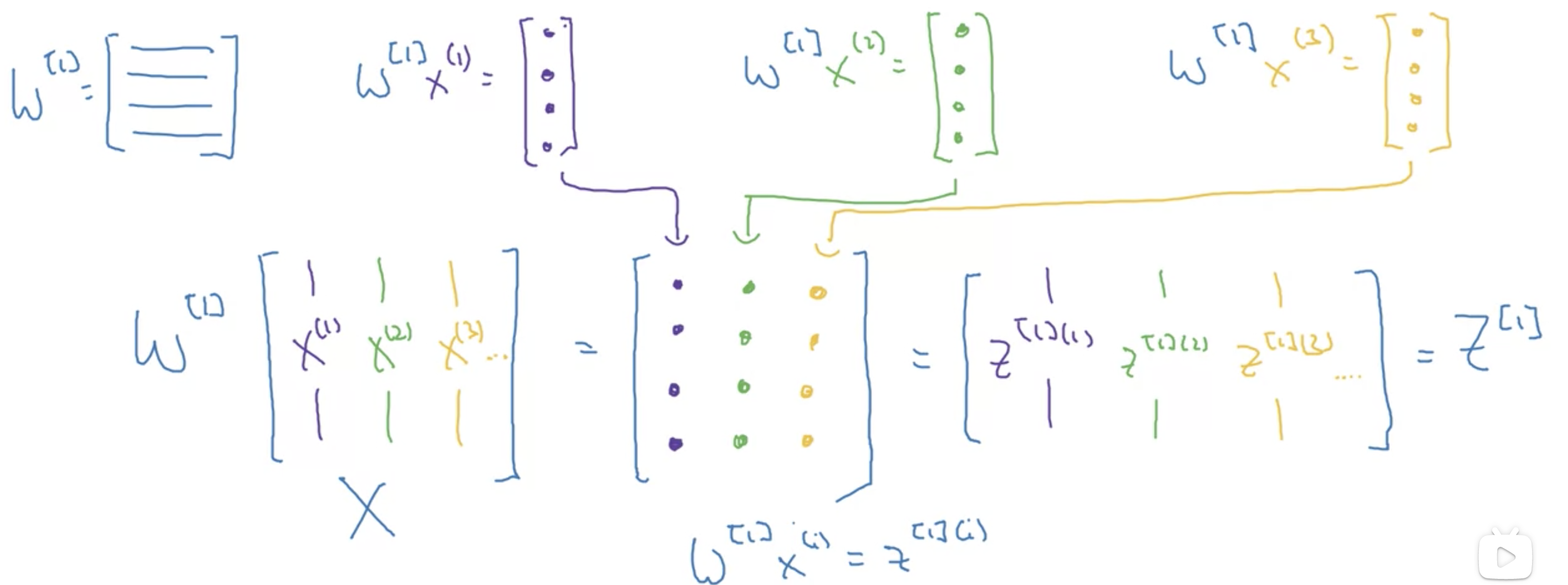
神经网络的运算及其向量化

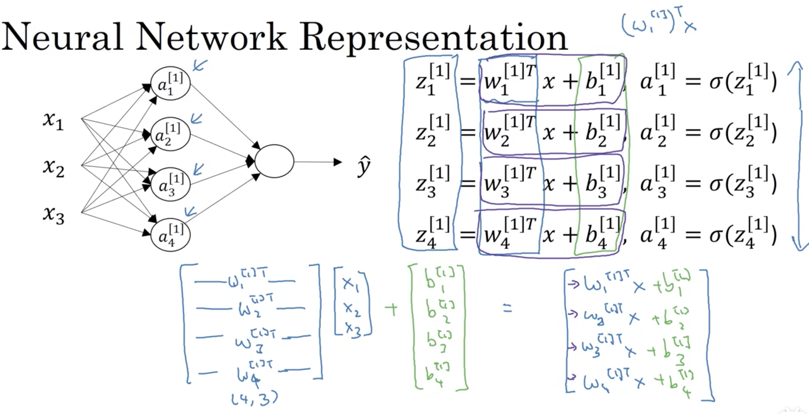
理解上图中的是不难的. 由每个WiTX都是对输入x1 ~ x3的线性组合得到一个输出Zi , 而且输出Z保持和输入X同为列向量(其元素是行向量)…可知输出的尺寸.

激活函数(详细内容见后续)

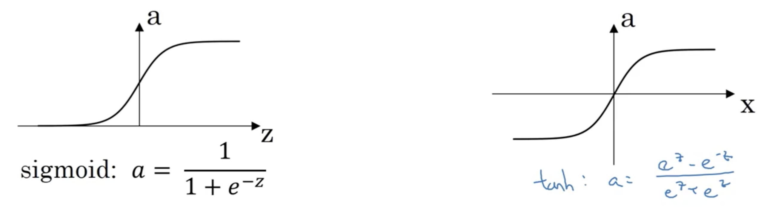
上图, sigmoid和Tanh.

从数值优化上讲, 激活函数至少要是非线性的.
对于二分类任务, 建议隐藏层使用Tanh,relu等激活函数, 仅仅在输出层上使用Sigmoid激活函数(注: 多分类任务上用softmax替代Sigmoid).

• 从数值优化上讲, Tanh总是比sigmoid更优秀, 为什么呢? 答: 因为Tanh会使得数值的均值趋于0, 这会使得下一层更容易训练…另外, tanh在特征相差明显时的效果会很好，在循环过程中会不断扩大特征效果.
• 从语义上讲, 用sigmoid表达概率值的作用是肯定的

sigmoid和TanH的共同缺点: 两边的梯度很低, 有梯度消失问题.

上图: relu和leakyrelu

relu和leakyrelu解决了Tanh和sigmoid的关于梯度的缺点, leakyrelu相比relu解决了z<0时的神经元死亡问题.
目前, relu和leakyrelu被主流所推荐使用.

参数随机初始化

w = np.random.randn(…) * 缩小系数. b = np.zero(…)
对于浅层网络(深层另做讨论), 缩小系数一般取0.01, 原因是我们希望该层计算出的z能接近0,以在大部分激活函数下都能确定很好的学习梯度.

解释一个误区: 权重不能被初始化为0的原因(哪怕只有一层被初始化为0), 并不是以为你输出z=0, 而是因为”对称失效问题”, 这将导致该隐层的不同神经元都肩负着相同的计算功能, 这种影响又将作用之后的神经元上, 进而导致网络学得一般. 其实, 随机初始化也是解决上述”对称失效问题”的关键

为什么网络的”深度”是有效的?

上图, 从提取低级信息—>到提取更高级信息的角度给出直观解释. 另外, “深度”比’宽度”更容易计算

正向与反向传播的细节

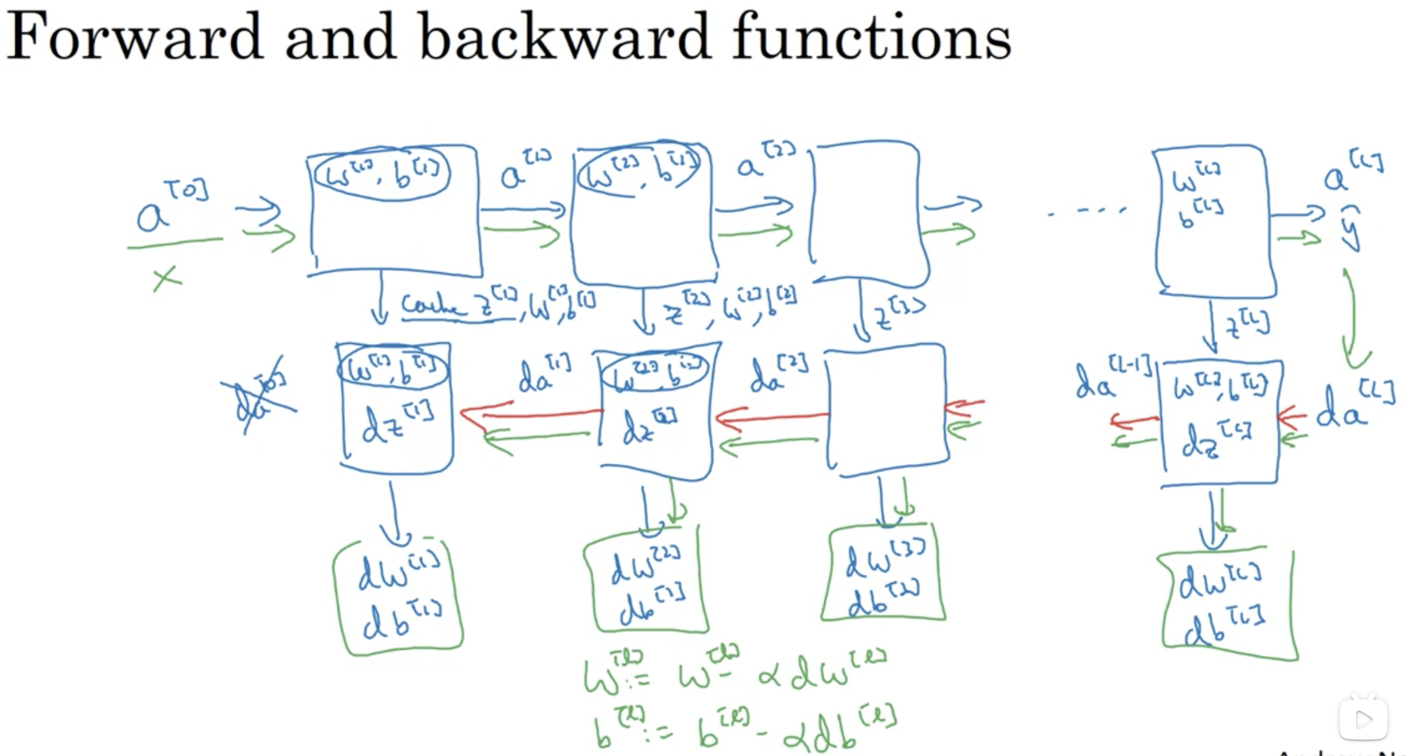
上图: 蓝色为正向传播, 红色为反向传播. 绿色代表一次梯度下降.

上方的图, 在正向传播的同时要缓存Z, 目的是后续计算反向传播. 其实很简单, 如下图, 在反向传播中, 我们求梯度的顺序.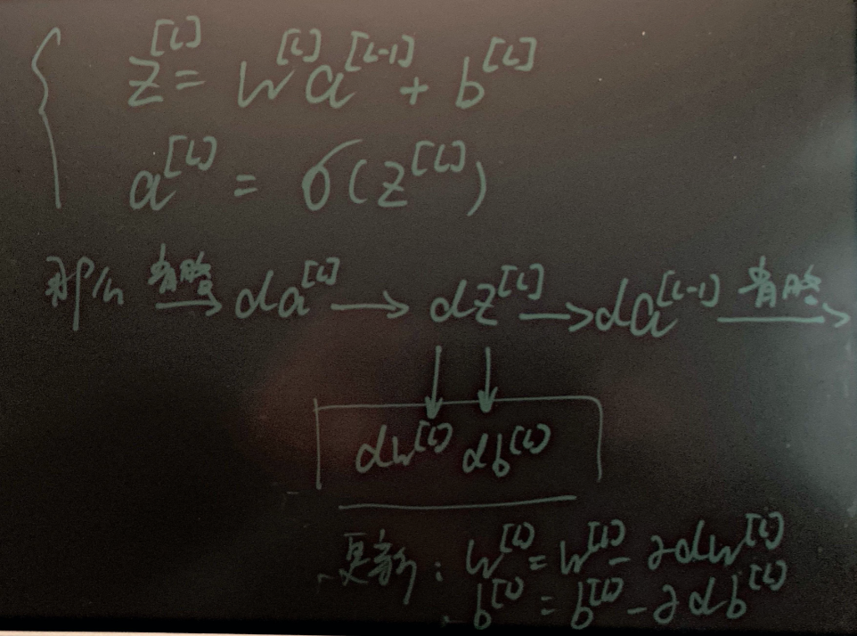

下面是正向传播的代码, 其返回正向传播输出A的同时, 还返回了Z的缓存

# GRADED FUNCTION: forward_propagation
def forward_propagation(X, parameters):
    """
    Argument:
    X -- input data of size (n_x, m)
    parameters -- python dictionary containing your parameters (output of initialization function)
    Returns:
    A2 -- The sigmoid output of the second activation
    cache -- a dictionary containing "Z1", "A1", "Z2" and "A2"
    """
    # Retrieve each parameter from the dictionary "parameters"
    ### START CODE HERE ### (≈ 4 lines of code)
    W1 = parameters["W1"]
    b1 = parameters["b1"]
    W2 = parameters["W2"]
    b2 = parameters["b2"]
    ### END CODE HERE ###
    # Implement Forward Propagation to calculate A2 (probabilities)
    ### START CODE HERE ### (≈ 4 lines of code)
    Z1 = np.dot(W1,X) + b1
    A1 = np.tanh(Z1)
    Z2 = np.dot(W2,A1) + b2
    A2 = sigmoid(Z2)
    ### END CODE HERE ###
    assert(A2.shape == (1, X.shape[1]))
    cache = {"Z1": Z1,
             "A1": A1,
             "Z2": Z2,
             "A2": A2}
    return A2, cache

浅层神经网络的numpy实现

源代码地址

• 1. 随机初始化参数….返回W和b矩阵

     # GRADED FUNCTION: initialize_parameters
     def initialize_parameters(n_x, n_h, n_y):
     """
     Argument:
     n_x -- size of the input layer
     n_h -- size of the hidden layer
     n_y -- size of the output layer
     
     Returns:
     params -- python dictionary containing your parameters:
                    W1 -- weight matrix of shape (n_h, n_x)
                    b1 -- bias vector of shape (n_h, 1)
                    W2 -- weight matrix of shape (n_y, n_h)
                    b2 -- bias vector of shape (n_y, 1)
     """
     
     np.random.seed(2) # we set up a seed so that your output matches ours although the initialization is random.
     
     ### START CODE HERE ### (≈ 4 lines of code)
     W1 = np.random.randn(n_h,n_x) * 0.01
     b1 = np.zeros((n_h,1))
     W2 = np.random.randn(n_y,n_h) * 0.01
     b2 = np.zeros((n_y,1))
     ### END CODE HERE ###
     
     assert (W1.shape == (n_h, n_x))
     assert (b1.shape == (n_h, 1))
     assert (W2.shape == (n_y, n_h))
     assert (b2.shape == (n_y, 1))
     
     parameters = {"W1": W1,
                  "b1": b1,
                  "W2": W2,
                  "b2": b2}
     
     return parameters
     

• 1. 一次正向传播…计算Z = WTX , A = sigmoid(Z), 返回 (A, Z) ```python

     GRADED FUNCTION: forward_propagation

def forward_propagation(X, parameters): “”” Argument: X — input data of size (n_x, m) parameters — python dictionary containing your parameters (output of initialization function)

Returns:
A2 -- The sigmoid output of the second activation
cache -- a dictionary containing "Z1", "A1", "Z2" and "A2"
"""
# Retrieve each parameter from the dictionary "parameters"
### START CODE HERE ### (≈ 4 lines of code)
W1 = parameters["W1"]
b1 = parameters["b1"]
W2 = parameters["W2"]
b2 = parameters["b2"]
### END CODE HERE ###

# Implement Forward Propagation to calculate A2 (probabilities)
### START CODE HERE ### (≈ 4 lines of code)
Z1 = np.dot(W1,X) + b1
A1 = np.tanh(Z1)
Z2 = np.dot(W2,A1) + b2
A2 = sigmoid(Z2)
### END CODE HERE ###

assert(A2.shape == (1, X.shape[1]))

cache = {"Z1": Z1,
         "A1": A1,
         "Z2": Z2,
         "A2": A2}

return A2, cache

- 3. 代价函数(逻辑回归)...计算CrossEntropyLoss(predictions, labels)...返回cost
```python
# GRADED FUNCTION: compute_cost

def compute_cost(A2, Y, parameters):
    """
    Computes the cross-entropy cost given in equation (13)

    Arguments:
    A2 -- The sigmoid output of the second activation, of shape (1, number of examples)
    Y -- "true" labels vector of shape (1, number of examples)
    parameters -- python dictionary containing your parameters W1, b1, W2 and b2

    Returns:
    cost -- cross-entropy cost given equation (13)
    """

    m = Y.shape[1] # number of example

    # Compute the cross-entropy cost
     ### START CODE HERE ### (≈ 2 lines of code)
    logprobs = Y*np.log(A2) + (1-Y)* np.log(1-A2)
    cost = -1/m * np.sum(logprobs)
    ### END CODE HERE ###

    cost = np.squeeze(cost)     # makes sure cost is the dimension we expect. 
                                # E.g., turns [[17]] into 17 
    assert(isinstance(cost, float))

    return cost

• 1. 一次反向传播(逻辑回归)(最难数学的一部分)…返回w和b的grads字典 ```python

     GRADED FUNCTION: backward_propagation

def backward_propagation(parameters, cache, X, Y): “”” Implement the backward propagation using the instructions above.

Arguments:
parameters -- python dictionary containing our parameters 
cache -- a dictionary containing "Z1", "A1", "Z2" and "A2".
X -- input data of shape (2, number of examples)
Y -- "true" labels vector of shape (1, number of examples)

Returns:
grads -- python dictionary containing your gradients with respect to different parameters
"""
m = X.shape[1]

# First, retrieve W1 and W2 from the dictionary "parameters".
### START CODE HERE ### (≈ 2 lines of code)
W1 = parameters["W1"]
W2 = parameters["W2"]
### END CODE HERE ###

# Retrieve also A1 and A2 from dictionary "cache".
### START CODE HERE ### (≈ 2 lines of code)
A1 = cache["A1"]
A2 = cache["A2"]
### END CODE HERE ###

# Backward propagation: calculate dW1, db1, dW2, db2. 
### START CODE HERE ### (≈ 6 lines of code, corresponding to 6 equations on slide above)
dZ2= A2 - Y
dW2 = 1 / m * np.dot(dZ2,A1.T)
db2 = 1 / m * np.sum(dZ2,axis=1,keepdims=True)
dZ1 = np.dot(W2.T,dZ2) * (1-np.power(A1,2))
dW1 = 1 / m * np.dot(dZ1,X.T)
db1 = 1 / m * np.sum(dZ1,axis=1,keepdims=True)
### END CODE HERE ###

grads = {"dW1": dW1,
         "db1": db1,
         "dW2": dW2,
         "db2": db2}

return grads

- 5. 更新W和b参数...计算w = w - lr*dw....返回parameters
```python
# GRADED FUNCTION: update_parameters

def update_parameters(parameters, grads, learning_rate = 1.2):
    """
    Updates parameters using the gradient descent update rule given above

    Arguments:
    parameters -- python dictionary containing your parameters 
    grads -- python dictionary containing your gradients 

    Returns:
    parameters -- python dictionary containing your updated parameters 
    """
    # Retrieve each parameter from the dictionary "parameters"
    ### START CODE HERE ### (≈ 4 lines of code)
    W1 = parameters["W1"]
    b1 = parameters["b1"]
    W2 = parameters["W2"]
    b2 = parameters["b2"]
    ### END CODE HERE ###

    # Retrieve each gradient from the dictionary "grads"
    ### START CODE HERE ### (≈ 4 lines of code)
    dW1 = grads["dW1"]
    db1 = grads["db1"]
    dW2 = grads["dW2"]
    db2 = grads["db2"]
    ## END CODE HERE ###

    # Update rule for each parameter
    ### START CODE HERE ### (≈ 4 lines of code)
    W1 = W1 - learning_rate * dW1
    b1 = b1 - learning_rate * db1
    W2 = W2 - learning_rate * dW2
    b2 = b2 - learning_rate * db2
    ### END CODE HERE ###

    parameters = {"W1": W1,
                  "b1": b1,
                  "W2": W2,
                  "b2": b2}

    return parameters

• 1. 建立你的神经网络模型…集成之前1~6的函数, 并以正确的顺序组合进行构建…返回parameters learnt by the model ```python

     GRADED FUNCTION: nn_model

def nn_model(X, Y, n_h, num_iterations = 10000, print_cost=False): “”” Arguments: X — dataset of shape (2, number of examples) Y — labels of shape (1, number of examples) n_h — size of the hidden layer num_iterations — Number of iterations in gradient descent loop print_cost — if True, print the cost every 1000 iterations

Returns:
parameters -- parameters learnt by the model. They can then be used to predict.
"""

np.random.seed(3)
n_x = layer_sizes(X, Y)[0]
n_y = layer_sizes(X, Y)[2]

# Initialize parameters, then retrieve W1, b1, W2, b2. Inputs: "n_x, n_h, n_y". Outputs = "W1, b1, W2, b2, parameters".
### START CODE HERE ### (≈ 5 lines of code)
parameters = initialize_parameters(n_x, n_h, n_y)
W1 = parameters["W1"]
b1 = parameters["b1"]
W2 = parameters["W2"]
b2 = parameters["b2"]
### END CODE HERE ###

# Loop (gradient descent)

for i in range(0, num_iterations):

    ### START CODE HERE ### (≈ 4 lines of code)
    # Forward propagation. Inputs: "X, parameters". Outputs: "A2, cache".
    A2, cache = forward_propagation(X, parameters)

    # Cost function. Inputs: "A2, Y, parameters". Outputs: "cost".
    cost = compute_cost(A2, Y, parameters)

    # Backpropagation. Inputs: "parameters, cache, X, Y". Outputs: "grads".
    grads = backward_propagation(parameters, cache, X, Y)

    # Gradient descent parameter update. Inputs: "parameters, grads". Outputs: "parameters".
    parameters = update_parameters(parameters, grads)

    ### END CODE HERE ###

    # Print the cost every 1000 iterations
    if print_cost and i % 1000 == 0:
        print ("Cost after iteration %i: %f" %(i, cost))

return parameters

- 7. 进行预测...集成正向传播....输入parameters和输入X, 返回正向传播的结果(即predictions)
```python
# GRADED FUNCTION: predict

def predict(parameters, X):
    """
    Using the learned parameters, predicts a class for each example in X

    Arguments:
    parameters -- python dictionary containing your parameters 
    X -- input data of size (n_x, m)

    Returns
    predictions -- vector of predictions of our model (red: 0 / blue: 1)
    """

    # Computes probabilities using forward propagation, and classifies to 0/1 using 0.5 as the threshold.
  ### START CODE HERE ### (≈ 2 lines of code)
    A2, cache = forward_propagation(X, parameters)
    predictions = np.round(A2)
    ### END CODE HERE ###

    return predictions