Linear fitting
function [a b]=linearfit(x,y)n=length(x);x2=x.*x;xy=x.*y;sx=sum(x);sy=sum(y);sxy=sum(xy);sx2=sum(x2);d=n*sx2-sx*sx;a=(sy*sx2-sx*sxy)/d;b=(n*sxy-sx*sy)/d;end%save as linearfit.m
Execute with
format long;
x=[0.5 1.2 2.1 2.9 3.6 4.5 5.7];
y=[2.81 3.24 3.80 4.30 4.73 5.29 6.03];
[a b]=linearfit(x,y);
c=[b a];
x1=0:0.1:6;
y1=polyval(c,x1);
figure(1);
set(gca, 'FontSize',16);
plot(x1,y1,x,y,'o');
xlabel('x');
ylabel('y');
title('dnm');
text(1,6,['a=', num2str(a)]);
text(1,5,['b=', num2str(b)]);
解释:num2str (Numer to String)用在表格中,以将数变成字符串方便显示;
polyval (Polynomial evaluation) polyval(p,x),其中p为系数矩阵,从高位到低位排列。
gives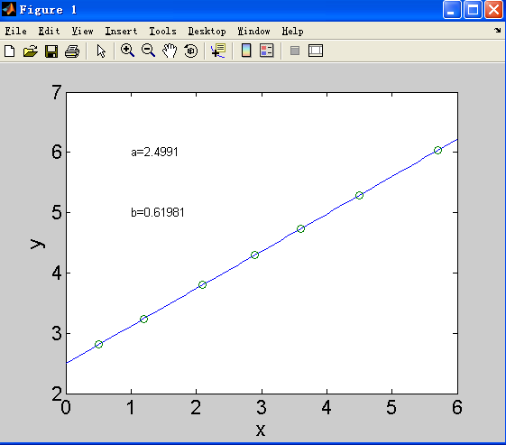
Exponential fitting
Execute with
clear all;
format long;
x=1:8;
y=[15.3 20.5 27.4 36.6 49.1 65.6 87.8 117.6];
yt=log(y);
xt=x;
[at bt]=linearfit(xt,yt);
a=exp(at);
b=bt;
x1=1:0.1:8;
y1=a*exp(b*x1);
figure(1);
set(gca,'FontSize',16);
plot(x1,y1,x,y,'o');
xlabel('x');
ylabel('y');
text(1,80,['a=' num2str(a)]);
text(1,70,['b=' num2str(b)]);
其中linearfit.m程序见 Linear fitting
gievs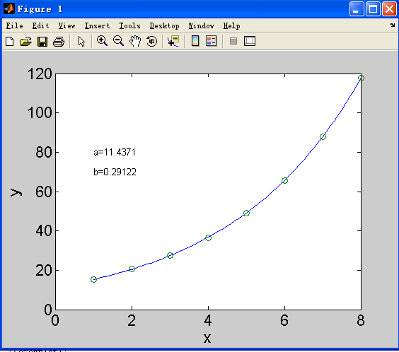 e
e
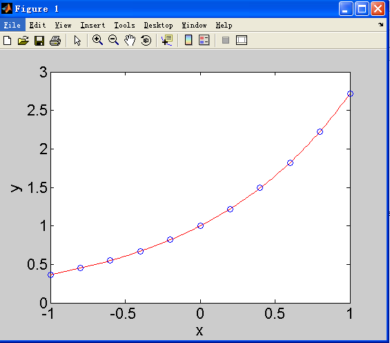
Polynomial regression
function a=polyreg(x,y,m)
n=length(x);
c(1:(2*m+1))=0;
T(1:(m+1))=0;
for j=1:(2*m+1)
    for k=1:n
        c(j)=c(j)+x(k)^(j-1);
        if(j<(m+2))
            T(j)=T(j)+y(k)*x(k)^(j-1);
        end
    end
end
S(1,:)=c(1:(m+1));
for k=2:(m+1)
    S(k,:)=c(k:(m+k));
end
a=S\T';
Execute with
clear all;
format long;
x=-1:0.2:1;
y=exp(x);
m=5;
a=polyreg(x,y,m);
c=[a(6) a(5) a(4) a(3) a(2) a(1)];
x1=-1:0.02:1;
y1=polyval(c,x1);
figure(1);
set(gca,'FontSize',16);
plot(x1,y1,'r',x,y,'o');
xlabel('x');
ylabel('y');
gird on;
Interpolant fitting
function v=lag(x,y,u)
n=length(x);
v=zeros(size(u));
for k=1:n
    w=ones(size(u));
    for j=[1:k-1 k+1:n]
        w=(u-x(j))./(x(k)-x(j)).*w;
    end
    v=v+w*y(k);
end

%save as lag.m
execute with
x = [0 pi/3 pi/2 2*pi/3 pi 4*pi/3 3*pi/2 5*pi/3 2*pi];
y = [0 sqrt(3)/2 1 sqrt(3)/2 0 -sqrt(3)/2 -1 -sqrt(3)/2 0];
u=0:0.05:2*pi;
v=lag(x,y,u);
figure(1);
plot(x,y,'bo',u,v,'black--','Linewidth',2)
grid on;
xlabel('x');
ylabel('y');
plot中,bo(Blue-O):xy的点用blue蓝色表示,o表示样子像一个圈儿O;black表示黑色,—代表虚线,不写两杠—的话默认实线,啥都不写默认蓝色实线。
可以通过改变u的步阶(increments)来让图更加丝滑或骨感。
gives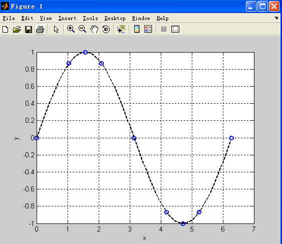
Matlab function _interpl1 _fitting
Simply execute
x=[-1.:0.2:1.];
y=1./(1.+x.*x);
xq=[-1.:0.05:1.];
v=interp1(x,y,xq);
figure(1);
plot(x,y,'o',xq,v,':.');
xlim([-1 1]);
where interpl1 is a matlab function, gives: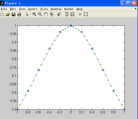

若有收获,就点个赞吧
0 人点赞
