WGCNA简介
hdWGCNA(scWGCNA)
single-cell analysis package
plotting and data science packages
co-expression network analysis packages:
using the cowplot theme for ggplot
set random seed for reproducibility
- 测试数据
为WGCNA设定seurat对象
构建metacell
construct metacells in each group
normalize metacell expression matrix:
- 基因共表达网络分析
  - 设置表达矩阵
— 选择多个分组 —————-
- 构建共表达网络

WGCNA简介

https://cloud.tencent.com/developer/article/1936465

hdWGCNA(scWGCNA)

单细胞WGCNA
github: https://github.com/smorabit/hdWGCNA
目前并非稳定版本！(2022-5-7)

安装

# install BiocManager
install.packages("BiocManager")
# install Bioconductor core packages
BiocManager::install()
# install additional packages:
install.packages(c("Seurat", "WGCNA", "igraph", "devtools"))
devtools::install_github('smorabit/hdWGCNA', ref='dev')
# test
library(hdWGCNA)

测试数据

# 作者提供测试数据
wget https://swaruplab.bio.uci.edu/public_data/Zhou_2020.rds
# pbmc3k测试数据(使用该数据)
wget https://cf.10xgenomics.com/samples/cell/pbmc3k/pbmc3k_filtered_gene_bc_matrices.tar.gz

输入数据要求

输入数据必须经过seurat或scanpy流程分析，以seurat为例子，输入数据必须经过以下分析

数据保存为seurat格式
基因表达矩阵需要经过归一化处理(NormalizeData)
确定了高变基因 VariableFeatures.
标准化的基因表达矩阵 ScaleData
RUNPCA，如需矫正批次效应使用RunHarmony
非线性降维 RunUMAP
cell聚类(FindNeighbors and FindClusters).
载入依赖
```r
single-cell analysis package
library(Seurat)

plotting and data science packages

library(tidyverse) library(cowplot) library(patchwork)

co-expression network analysis packages:

library(WGCNA) library(hdWGCNA)

using the cowplot theme for ggplot

theme_set(theme_cowplot())

set random seed for reproducibility

set.seed(12345)

<a name="QQfsL"></a>
### 读入数据
<a name="aV2Qc"></a>
#### 基本分析
```r
pbmc.data <- Read10X(data.dir = "./data/pbmc3k")
pbmc <- CreateSeuratObject(counts = pbmc.data,project = "pbmc3k",min.cells = 3,min.features = 200)
pbmc[["percent.mt"]] <- PercentageFeatureSet(pbmc,pattern = "^MT-")
pbmc <- subset(pbmc,subset = nFeature_RNA > 200 & nFeature_RNA < 2500 & percent.mt < 5)
pbmc <- NormalizeData(pbmc,normalization.method = "LogNormalize",scale.factor = 10000)
pbmc <- FindVariableFeatures(pbmc,selection.method = "vst",nfeatures = 2000)
pbmc <- ScaleData(pbmc, vars.to.regress = "percent.mt")
pbmc <- ScaleData(pbmc,features = VariableFeatures(pbmc))
pbmc <- RunPCA(pbmc)
pbmc <- FindNeighbors(pbmc,dims = 1:13)
pbmc <- FindClusters(pbmc,resolution = 0.5)
pbmc <- RunTSNE(pbmc,dims = 1:13)
pbmc <- RunUMAP(pbmc,dims = 1:13)
new.cluster.ids <- c("Naive CD4 T", "CD14+ Mono", "Memory CD4 T", "B", "CD8 T", "FCGR3A+ Mono",
    "NK", "DC", "Platelet")
names(new.cluster.ids) <- levels(pbmc)
pbmc <- RenameIdents(pbmc, new.cluster.ids)
pbmc@meta.data$cell_type <- Idents(pbmc)

测试数据

p <- DimPlot(seurat_obj, group.by='cell_type', label=TRUE) +
   umap_theme() + ggtitle('Zhou et al Control Cortex') + NoLegend()
p

为WGCNA设定seurat对象

hdWGCNA的结果储存在seurat对象的@miscslot中，一个seurat对象可以存在多个hdWGCNA experiment
使用SetupForWGCNA 设定seurat对象, 此步骤可以设定 scWGNCA experiment的名称和选择使用哪些符合条件的基因，主要有三种方法可以筛选基因，通过gene_select 选项指定，wgcna_name指定名称

variable: 使用seurat确定的VariableFeatures
fraction: use genes that are expressed in a certain fraction of cells for in the whole dataset or in each group of cells, specified by group.by.根据基因在多少比例的cell中表达的阈值筛选基因
custom: 自行指定gene列表
```
pbmc <- SetupForWGCNA(
pbmc,
gene_select = "fraction", # the gene selection approach
fraction = 0.05, # fraction of cells that a gene needs to be expressed in order to be included
wgcna_name = "tutorial" # the name of the hdWGCNA experiment
)
```
查看一下@misc
```
pbmc@misc # list
#out
$active_wgcna
'tutorial'
$tutorial
$wgcna_group
'all'
$wgcna_genes
'AL627309.1''LINC01409'...
```
构建metacell
设定了seurat对象后，第一步是构建metacell, 所有metacell是来自相同生物样品的一小组相似细胞的聚类，scWGCNA使用了KNN算法识别相似的cell, 将cell聚类后再计算基因的平均表达量，得到metacell的基因表达矩阵，大大降低了原始矩阵的稀疏性
使用MetacellsByGroups构建metacell, 该函数创建了一个新的 Seurat 对象 ```r
construct metacells in each group
pbmc <- MetacellsByGroups( seurat_obj = pbmc, group.by = “cell_type”, # specify the columns in seurat_obj@meta.data to group by k = 25, # nearest-neighbors parameter ident.group = ‘cell_type’ # set the Idents of the metacell seurat object )

normalize metacell expression matrix:

pbmc <- NormalizeMetacells(pbmc)

`seurat_obj`: seurat对象<br />`**group.by**`**: **确定将在哪些组中构建metacell，可以指定多个，名称要和`seurat_obj@meta.data`一致<br />`k`: KNN算法的k值, 一般设定在25 - 75之间, 本例有40,039 个cell，每个生物样本中的细胞数从 890 - 8188 不等<br />`ident.group`: Idents of the metacell seurat object
<a name="i0FVQ"></a>
#### 对构建好的metacell进行标准流程分析:可选
使用 `GetMetacellObject`可以提取metacell对象
```r
metacell_obj <- GetMetacellObject(pbmc)
## 查看cell数量
metacell_obj
An object of class Seurat 
36601 features across 21058 samples within 1 assay 
Active assay: RNA (36601 features, 0 variable features)
pbmc
An object of class Seurat 
36601 features across 36671 samples within 1 assay 
Active assay: RNA (36601 features, 0 variable features)
 2 dimensional reductions calculated: harmony, umap

hdWGCNA封装了部分标准流程的步骤可直接调用，支持%>%

pbmc <- pbmc %>%
  NormalizeMetacells() %>%
  ScaleMetacells(features=VariableFeatures(seurat_obj)) %>%
  RunPCAMetacells(features=VariableFeatures(seurat_obj)) %>%
  RunHarmonyMetacells(group.by.vars='Sample') %>%
  RunUMAPMetacells(reduction='harmony', dims=1:15)
p1 <- DimPlotMetacells(pbmc, group.by='cell_type') + umap_theme + ggtitle("Cell Type")
p2 <- DimPlotMetacells(pbmc, group.by='Sample') + umap_theme + ggtitle("Sample")
p1 | p2

基因共表达网络分析

对数据集中的抑制性神经元 (INH) 细胞执行基因共表达网络分析

设置表达矩阵

使用SetDatExpr()设置表达矩阵，该函数包括了提取子集和转置矩阵的功能, 关键参数如下

seurat_obj: seurat对象名称
group_name：需要分析哪部分cell(需要分析的cell的分组名)，名称应在group.by指定的范围内
use_metacells: 是否使用metacell
group.by: 根据seurat@metada哪一列分组 ```r pbmc <- SetDatExpr( pbmc, group_name = “NK”, # the name of the group of interest in the group.by column group.by=’cell_type’ # the metadata column containing the cell type info. This same column should have also been used in MetacellsByGroups )

— 选择多个分组 —————-

pbmc <- SetDatExpr( pbmc, group_name = c(“CD8 T”, “B”), group.by=’cell_type’ )

<a name="kz58Y"></a>
#### 选择软阈值
使用`TestSoftPowers()`函数确定软阈值，`PlotSoftPowers()`可视化结果, 如果前面没有进行`SetDatExpr`，可以再此步骤执行，参数和`SetDatExpr()`函数一致，WGCNA 和 hdWGCNA 的一般模型拟合大于或等于 0.8时的最低软阈值。本例给出的是7
```r
# Test different soft powers:
pbmc <- TestSoftPowers(
  pbmc,
  setDatExpr = FALSE, # set this to FALSE since we did this above
)
# 可视化软阈值结果
plot_list <- PlotSoftPowers(pbmc)
# assemble with patchwork
wrap_plots(plot_list, ncol=2)

使用[GetPowerTable](../reference/GetPowerTable.html)()可以获取具体的软阈值表格

power_table <- GetPowerTable(pbmc)
head(power_table, 3)
###
Power    SFT.R.sq      slope truncated.R.sq   mean.k. median.k.    max.k.
1     1 0.192964167 10.1742363      0.9508966 5887.9290 5901.7852 6501.0283
2     2 0.001621749  0.4801145      0.9828730 3092.6379 3092.7878 3835.2202
3     3 0.150812707 -3.2345892      0.9918393 1657.6198 1646.6169 2349.6967

构建共表达网络

使用ConstructNetwork()构建基因共表达网络

# construct co-expression network:
pbmc <- ConstructNetwork(
  pbmc, 
  soft_power=12,
  setDatExpr=FALSE
)

使用PlotDendrogram()可视化

PlotDendrogram(pbmc, main='pbmc3k hdWGCNA')

模块特征基因(MEs)

相应模块的表达矩阵的第一主成分，代表了该模块内基因表达的整体水平。因此，模块特征基因并非某个具体的基因，而是一种“特征组合”
使用ModuleEigengenes()计算模块特征基因, 可能会报错

Error in data.use %*% cell.embeddings : non-conformable arguments
https://github.com/immunogenomics/harmony/issues/86
增加选项project.dim = F 解决

# compute all MEs in the full single-cell dataset
pbmc <- ModuleEigengenes(
 pbmc,
 group.by.vars="cell_type"
)

使用GetMEs()可以得到模块特征基因的表达矩阵，默认使用harmonized矫正，即得到hMEs

# harmonized module eigengenes:
hMEs <- GetMEs(pbmc)
 turquoise       blue     brown       grey     yellow
AAACATACAACCAC-1   4.885751  0.7222126 -2.035966 -4.5174804 -2.0320305
AAACATTGAGCTAC-1   2.331174 -0.5567514  3.371447  0.4035175 -0.7455446
# module eigengenes: 未矫正的数据
MEs <- GetMEs(pbmc, harmonized=FALSE)

模块间基因连通度计算

在共表达网络分析中，需要得到每个模块内高连接度的基因。使用ModuleConnectivity()确定每个基因的基于特征基因的连接性，也称为kME。
hdWGCNA includes the ModuleConnectivity to compute the kME values in the full single-cell dataset, rather than the metacell dataset. This function essentially computes pairwise correlations between genes and module eigengenes. kME can be computed for all cells in the dataset, but we recommend computing kME in the cell type or group that was previously used to run ConstructNetwork

# compute eigengene-based connectivity (kME):
seurat_obj <- ModuleConnectivity(
  seurat_obj,
  group.by = 'cell_type', group_name = 'NK'
)

使用GetModules()获取每个基因的kME信息

modules <- GetModules(pbmc)

计算gene signature score

使用ModuleExprScore计算每个模块的gene signature score, 支持UCell和Seurat的算法

# compute gene scoring for the top 25 hub genes by kME for each module
# with Seurat method
pbmc <- ModuleExprScore(
  pbmc,
  n_genes = 25,
  method='Seurat'
)
# compute gene scoring for the top 25 hub genes by kME for each module
# with UCell method
library(UCell) # R version >= 4.1
pbmc <- ModuleExprScore(
  pbmc,
  n_genes = 25,
  method='UCell'
)
saveRDS(pbmc, file='./data/pbmc3kwgcna.rds')

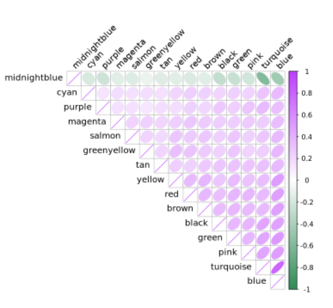
模块间相关性

library(corrplot)
ModuleCorrelogram(pbmc)

# use GGally to investigate 6 selected modules:
GGally::ggpairs(GetMEs(pbmc)[,c(1:3,12:15)])

scRNA data analysis

scRNA-hdWGCNA

WGCNA简介

hdWGCNA(scWGCNA)

安装

测试数据

输入数据要求

载入依赖

single-cell analysis package

plotting and data science packages

co-expression network analysis packages:

using the cowplot theme for ggplot

set random seed for reproducibility

测试数据

为WGCNA设定seurat对象

构建metacell

construct metacells in each group

normalize metacell expression matrix:

基因共表达网络分析

设置表达矩阵

— 选择多个分组 —————-

构建共表达网络

模块特征基因(MEs)

模块间基因连通度计算

计算gene signature score

模块间相关性