【考前提醒】：

1.导入数据后先对数据进行简单的观察，行列数，数据类型，每行每列含义，在进行计算
2.不要只会埋头敲代码，要明白每一步是在做什么，有结果后，要学会对其进行简单的检查，看命令有没有错误
3.报错时，要冷静分析错误的原因，不要一味重复进行，没有用的

2021年生统作业

第一次作业

1.计算平均数

2.计算概率

3.P(A+B)=P(A)+P(B)-P(AB)

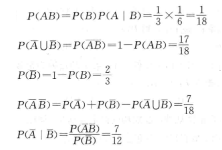
4.P(AB)=P(A)P(B|A)=P(B)P(A|B)

5.中心极限定理

第二次作业

1.z检验

2.概率计算

3.比例检验

4.泊松逼近

5.概率计算

6.标准正态化

第三次作业

1.R 的基本操作

#查看当前工作目录；更改工作目录到桌面
> getwd()
> setwd('C:/Users/cuihy/Desktop/')
#下载安装 R 包
> install.packages('datasets')
> library(datasets)
#载入 iris 数据集，并查看数据行列数，查看数据类型
> data("iris")
> nrow(iris)
> ncol(iris)
> mode(iris) 或 class(iris) 或 str(iris)
#对 iris 的 Sepal.Length 进行描述统计。并绘制箱线图。
> summary(iris$sepal_length)
> boxplot(iris$sepal_length)
#用 R 查看 t.test()的帮助文档
> ?t.test

2.t.检验

#利用上一题的鸢尾花数据集进行计算。鸢尾花的平均花瓣长度为 3.5cm，这种说法正确吗？
> t.test(iris$Sepal.Length,alternative = "two.sided",mu = 3.5)
    One Sample t-test
data:  iris$Sepal.Length
t = 34.659, df = 149, p-value < 2.2e-16
alternative hypothesis: true mean is not equal to 3.5
95 percent confidence interval:
 5.709732 5.976934
sample estimates:
mean of x 
 5.843333

3.文件基本操作

#查看该目录下的文件
> dir()
#将基因表达数据 homework3.1_data.txt 导入到 R 中,使行名为样本编号，列名为 symbol 基因
名，并查看行列数及前 5 行数据, 计算每个基因表达的均值，标准差和最大值。
> data3 <- read.table("D:/郭东灵/我的研究生/生统作业/homework3.1_data.txt",header=TRUE,row.names=1)
> data3 <- t(data3)
> dim(data)
14 199
> head(data, n=5)
> statistic <- apply(data3,2,function(x){
+ Mean <- mean(x);names(Mean)<-"Mean"
+ Sd<-sd(x);names(Sd)<-"Sd"
+ Max<-max(x);names(Max)<-"Max"
+ return(c(Mean,Sd,Max))
+ })  ；apply函数行、列运算
#对样本 A9QA 的基因表达进行统计描述, 找出不表达的基因
> summary(data["A9QA",])
> names(data3["A9QA",which(data3["A9QA",]==0)]) ； names(向量)
> colnames(data3[,which(data3["A9QA",]==0)]) ； colnames(矩阵)
#从数据中随机选取 10 个基因得到新的表达矩阵，并绘制箱线图；
> samp <- data3[,sample(1:ncol(data3),10)] ； sample取随机数
> boxplot(samp)

4.大样本比例检验，故对答案存疑！

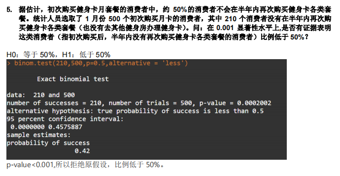
> z <- (210/500 - 0.5) / sqrt(0.25/500) ;z
[1] -3.577709
> pnorm(z)
[1] 0.0001733097
因p-value值<0.001，故拒绝原假设，比例低于50%

t检验

> time <- c(4.21, 5.55, 3.02, 5.13, 4.77, 2.34, 3.54, 3.2, 4.5, 6.1, 0.38, 5.12, 6.19, 3.79,1.08)
> shapiro.test(time)  #小样本要进行正态性检验
> t.test(time,alternative = "less",mu = 5)

第四次作业

1.秩检验

> wilcox.test(a,b,paired = FALSE,alternative = "two.sided",exact = FALSE)

2.方差相等的t检验

#检验方差是否同质
> var.test(a,b)
#t检验
> shapiro.test(a)
> shapiro.test(b)
> t.test(a,b,paired = FALSE,var.equal = TRUE)

3.单样本t-test【step-by-step】

H0:μ=4.15；Ha：μ≠4.15
> t <- (4.98-4.15)/(2.78/sqrt(16));t
[1] 1.194245
> p <- 2*(1-pt(t,15));p
[1] 0.2509263
因p>0.05，故接收原假设，即认为陈旧性心肌梗死患者的血浆载脂蛋白E平均浓度与正常人无显著差别有统计学意义
> left <- 4.98 - qt(0.975,15)*2.78/sqrt(16);left
[1] 3.498643
> right <- 4.98 + qt(0.975,15)*2.78/sqrt(16);right
[1] 6.461357
95%CI=[3.498643，6.461357]

第五次作业

1.ANOVA（step-by-step）

#读取数据
> group1<-c(243, 251, 275, 291, 347, 354, 380, 392)
> group2<-c(206, 210, 226, 249, 255, 273, 285, 295, 309)
> group3<-c(241, 258, 270, 293, 328)
> folic_acid <- data.frame(value=c(group1,group2,group3),cls=c(rep("G1",length(group1)),rep("G2",length(group2)),rep("G3",length(group3))))
> folic_acid <- transform(folic_acid,cls=factor(cls,levels = c("G1","G2","G3")))
> attach(folic_acid)
#正态性检验
> shapiro.test(group1)
> shapiro.test(group2)
> shapiro.test(group3)
#方差齐性检验
> bartlett.test(value~cls,folic_acid)
#step-by-step
#计算平方和
> GrandMean <- mean(folic_acid$value);GrandMean
> SMeans <- aggregate(folic_acid$value,by=list(folic_acid$cls),FUN=mean);SMeans
> SVars <- aggregate(folic_acid$value,by=list(folic_acid$cls),FUN=var);SVars
> SLens <- aggregate(folic_acid$value,by=list(folic_acid$cls),FUN=length);SLens
> within_SS <- sum((SLens$x-1)*SVars$x)
> total_SS <- sum((value-GrandMean)^2) 
> between_SS <- total_SS-within_SS
> df_between <- length(levels(cls))-1
> df_within <- length(value) - length(levels(cls))
> between_MS <- between_SS/df_between
> within_MS <- within_SS/df_within
> F_ration <- between_MS/within_MS
> P_value <- 1-pf(F_ration,df_between,df_within);P_value
[1] 0.04358933
因p_value<0.05，故拒绝原假设，即认为三组之间存在显著性差异

2.kruskal.test（R）（序数因变量）

注：数据格式转换 ```r

drug_data <- read.table(“D:/郭东灵/学习/生统/第五次/homework5_data2.csv”,header=TRUE,sep=”,”) View(drug_data) drug_data <-melt(drug_data） attach(drug_data) kruskal.test(value~variable,data=drug_data)

Kruskal-Wallis rank sum test

data: value by variable Kruskal-Wallis chi-squared = 3.0973, df = 2, p-value = 0.2125

<a name="bZrvV"></a>
### 3.单因素方差分析（R）
```r
> production <- read.table("D:/郭东灵/学习/生统/第五次/homework5_data3.txt",header=TRUE,colClass=c("numeric","factor"))
#正态性检验
> shapiro.test(production$yield[production$seed==1])
> shapiro.test(production$yield[production$seed==2])
> shapiro.test(production$yield[production$seed==3])
#齐性检验
> bartlett.test(yield~seed,data=production)
#方差分析
> summary(aov(yield~seed,data=production))
#后续分析
> pairwise.t.test(production$yield,production$seed,p.adjust.method = "fdr")
> TukeyHSD(aov(yield~seed,data=production))

4.双因素方差分析

> tooth <- read.table("D:/郭东灵/学习/生统/第五次/homework_5_data4.csv",sep=",",header=TRUE,colClass=c("numeric","factor","factor"))
> summary(tooth$len)
   Min. 1st Qu.  Median    Mean 3rd Qu.    Max. 
   4.20   13.07   19.25   18.81   25.27   33.90 
> summary(aov(len~supp*dose,data = tooth))
> TukeyHSD(aov(len~supp*dose,data = tooth))

第六次作业

1.多元线性回归分析

(1)

> Y <- c(162,120,223,131,67,167,81,192,116,55,252,232,144,103,212)
> X1 <- c(274,180,375,205,86,265,98,330,195,53,430,372,236,157,370)
> X2 <- c(2450,3250,3802,2838,2347,3782,3008,2450,2137,2560,4020,4427,2660,2088,2605)
> ff <- lm(Y~X1+X2)
> summary(ff)
Call:
lm(formula = Y ~ X1 + X2)
Residuals:
    Min      1Q  Median      3Q     Max 
-3.9014 -1.2923 -0.1171  1.6956  3.7601 
Coefficients:
            Estimate Std. Error t value Pr(>|t|)    
(Intercept) 3.984819   2.553039   1.561    0.145    
X1          0.496767   0.006360  78.104  < 2e-16 ***
X2          0.008913   0.001017   8.762 1.46e-06 ***
---
Signif. codes:  0 ‘***’ 0.001 ‘**’ 0.01 ‘*’ 0.05 ‘.’ 0.1 ‘ ’ 1
Residual standard error: 2.287 on 12 degrees of freedom
Multiple R-squared:  0.9988,    Adjusted R-squared:  0.9986 
F-statistic:  5142 on 2 and 12 DF,  p-value: < 2.2e-16

由此可得，Y =3.984819 + 0.496767X1 + 0.008913X2
从结果可得，F检验的p-value< 2.2e-16，且对X1和X2的t检验的p-value也都均显著，表明获得的线性回归方程有效

（2）

> newdata <- data.frame(x1=200,x2=3000)
> predict(ff,newdata = newdata,interval = "prediction",level = 0.95)
       fit      lwr      upr
1 130.0772 124.8931 135.2612

当X1=200，X2=3000时，根据预测的回归方程可得Y为130.0772

2.逻辑回归

（1）读数据

> install.packages("ISLR")
> library(ISLR)
> summary(Default)
 default    student       balance           income     
 No :9667   No :7056   Min.   :   0.0   Min.   :  772  
 Yes: 333   Yes:2944   1st Qu.: 481.7   1st Qu.:21340  
                       Median : 823.6   Median :34553  
                       Mean   : 835.4   Mean   :33517  
                       3rd Qu.:1166.3   3rd Qu.:43808  
                       Max.   :2654.3   Max.   :73554  
> View(Default)

该数据集中共有4个观测值。

（2）逻辑模型

> Default_training <- Default[1:7000,]
> fit_tr <- glm(default~student+balance+income,data = Default_training,family = binomial())
> summary(fit_tr)
Call:
glm(formula = default ~ student + balance + income, family = binomial(), 
    data = Default_training)
Deviance Residuals: 
    Min       1Q   Median       3Q      Max  
-2.1872  -0.1417  -0.0549  -0.0196   3.6863  
Coefficients:
              Estimate Std. Error z value Pr(>|z|)    
(Intercept) -1.101e+01  5.889e-01 -18.704   <2e-16 ***
studentYes  -6.464e-01  2.846e-01  -2.271   0.0231 *  
balance      5.829e-03  2.781e-04  20.958   <2e-16 ***
income       4.711e-06  9.875e-06   0.477   0.6333    
---
Signif. codes:  0 ‘***’ 0.001 ‘**’ 0.01 ‘*’ 0.05 ‘.’ 0.1 ‘ ’ 1
(Dispersion parameter for binomial family taken to be 1)
    Null deviance: 2090.7  on 6999  degrees of freedom
Residual deviance: 1109.4  on 6996  degrees of freedom
AIC: 1117.4
Number of Fisher Scoring iterations: 8

(3)简化模型

> fit_red <- glm(default~student+balance,data = Default_training,family = binomial())
> summary(fit_red)
Call:
glm(formula = default ~ student + balance, family = binomial(), 
    data = Default_training)
Deviance Residuals: 
    Min       1Q   Median       3Q      Max  
-2.2079  -0.1420  -0.0550  -0.0196   3.6762  
Coefficients:
              Estimate Std. Error z value Pr(>|z|)    
(Intercept) -1.083e+01  4.405e-01 -24.586  < 2e-16 ***
studentYes  -7.526e-01  1.763e-01  -4.268 1.97e-05 ***
balance      5.832e-03  2.781e-04  20.971  < 2e-16 ***
---
Signif. codes:  0 ‘***’ 0.001 ‘**’ 0.01 ‘*’ 0.05 ‘.’ 0.1 ‘ ’ 1
(Dispersion parameter for binomial family taken to be 1)
    Null deviance: 2090.7  on 6999  degrees of freedom
Residual deviance: 1109.6  on 6997  degrees of freedom
AIC: 1115.6
Number of Fisher Scoring iterations: 8
> anova(fit_red,fit_tr,test = "Chisq")
Analysis of Deviance Table
Model 1: default ~ student + balance
Model 2: default ~ student + balance + income
  Resid. Df Resid. Dev Df Deviance Pr(>Chi)
1      6997     1109.6                     
2      6996     1109.4  1  0.22749   0.6334

根据检验结果可知，卡方值(p=0.6334)不显著，表明两个模型拟合程度一样好，因此可以使用简化模型来进行解释。

（4）模型有效性

> Default_test <- Default[7001:10000,1:3]
> Default_test$prob <- predict(fit_red,newdata = Default_test,type = "response")
> summary(Default_test)
 default    student       balance            prob          
 No :2907   No :2105   Min.   :   0.0   Min.   :0.0000093  
 Yes:  93   Yes: 895   1st Qu.: 486.1   1st Qu.:0.0002745  
                       Median : 826.7   Median :0.0019506  
                       Mean   : 837.4   Mean   :0.0351620  
                       3rd Qu.:1168.0   3rd Qu.:0.0133454  
                       Max.   :2654.3   Max.   :0.9801269 
> Default_test <- Default_test[order(Default_test$prob,decreasing = TRUE),]
> Default_test[1:93,"prob"] <- "Yes"
> Default_test[94:3000,"prob"] <- "No"
> Default_test$prob <- factor(Default_test$prob,levels = c("Yes","No"),labels = c("Yes","No"))
> Default_test$judg <- ifelse(Default_test$default == Default_test$prob,1,0)
> table(Default_test$judg)
   0    1 
  90 2910 
> accuracy <- 2910/3000*100 ;accuracy
[1] 97

故，该训练模型的准确性为97%

3.线性回归

(1)多元线性回归

> crop_yield <- read.table("D:/郭东灵/学习/生统作业/第六次/homework6.3.csv",sep=",",header=TRUE)
> fit_crop <- lm(crop_yield~illumination_time+illumination_intensity+chemical_fertilizer,data = crop_yield)
> summary(fit_crop)
Call:
lm(formula = crop_yield ~ illumination_time + illumination_intensity + 
    chemical_fertilizer, data = crop_yield)
Residuals:
     Min       1Q   Median       3Q      Max 
-0.41065 -0.11562 -0.00984  0.13466  0.51361 
Coefficients:
                       Estimate Std. Error t value Pr(>|t|)    
(Intercept)              7.5891     2.4450   3.104 0.004567 ** 
illumination_time       -2.3577     0.6379  -3.696 0.001028 ** 
illumination_intensity   1.6122     0.2954   5.459 1.01e-05 ***
chemical_fertilizer      0.5012     0.1259   3.981 0.000491 ***
---
Signif. codes:  0 ‘***’ 0.001 ‘**’ 0.01 ‘*’ 0.05 ‘.’ 0.1 ‘ ’ 1
Residual standard error: 0.2347 on 26 degrees of freedom
Multiple R-squared:  0.8936,    Adjusted R-squared:  0.8813 
F-statistic:  72.8 on 3 and 26 DF,  p-value: 8.883e-13

（2）模型预测

> testdata$crop_yield <- predict(fit_crop,newdata = testdata)
> testdata
  illumination_time illumination_intensity chemical_fertilizer crop_yield
1                 0                      0                7.77   11.48305

经模型预测，施肥量7.77下黑暗生长的作物产量为11.48305kg

（3）计算R2以及F检验

> crop_yield$pred <- predict(fit_crop,newdata = crop_yield)
> Res_SS <- sum((crop_yield$crop_yield - crop_yield$pred)^2) ; Res_SS
[1] 1.431813
> Total_SS <- sum((crop_yield$crop_yield - mean(crop_yield$crop_yield))^2) ; Total_SS
[1] 13.45859
> Reg_SS <- Total_SS - Res_SS ; Reg_SS
[1] 12.02677
> R2 <- Reg_SS/Total_SS ; R2
[1] 0.8936135

H0：β1=β2=0  ；  Ha：β1、β2中至少有一个不等于0
> fit_crop_reduce <- lm(crop_yield~chemical_fertilizer,data = crop_yield)
> crop_yield$reduce <- predict(fit_crop_reduce,newdata = crop_yield)
> Res_SS_reduce <- sum((crop_yield$crop_yield - crop_yield$reduce)^2) ;Res_SS_reduce
[1] 3.131884
> Total_SS_reduce <- sum((crop_yield$crop_yield - mean(crop_yield$reduce))^2) ; Total_SS_reduce
[1] 13.45859
> Reg_SS_reduce <- Total_SS_reduce - Res_SS_reduce ; Reg_SS_reduce
[1] 10.3267
> Reg_df_reduce <- 2 ;Reg_df_reduce
[1] 2
> Res_df <- 30-3-1 ; Res_df
[1] 26
> Reg_MS_reduce <- Reg_SS_reduce / Reg_df_reduce ;Reg_MS_reduce
[1] 5.163351
> Res_MS <- Res_SS/Res_df ; Res_MS
[1] 0.05506972
> F <- Reg_MS_reduce / Res_MS ; F
[1] 93.76027
> 1-pf(F,Reg_df_reduce,Res_df)
[1] 1.294076e-12

可知，R2为0.8936135；且F检验的p-value（1.294076e-12）值远<0.01，故拒绝原假设，认为β1、β2中至少有一个不等于0

第七次作业

1.主成分分析

> data(iris)
> head(iris, 3)
> par(mfrow=c(2,2))   #将画幅进行分割
#绘制直方图
> hist(iris$Sepal.Length, breaks = 20)
> hist(iris$Sepal.Width, breaks = 20)
> hist(iris$Petal.Length, breaks = 20)
> hist(iris$Petal.Width, breaks = 20)
#取对数值
> log.iris <- log(iris[,1:4])
#主成分分析
> iris.pca <- prcomp(log.iris,center = TRUE,scale = TRUE )#center标准分布 #scale量纲标准化
> print(iris.pca)
> summary(iris.pca)
故，需要PC1，PC2

2.聚类分析

> iris.hc <- hclust(dist(iris[,1:4]))
> plot(iris.hc,hang = -1)
> re <- rect.hclust(iris.hc, k=3)#标注3类
> iris.id <- cutree(iris.hc, 3)#分类编号
> table(iris.id,iris$Species)
iris.id setosa versicolor virginica
      1     50          0         0
      2      0         23        49
      3      0         27         1

3.RNA-seq

> gene_data <- read.table("D:/郭东灵/学习/生统/第七次/homework7_data2.txt",header=TRUE)
#画密度图
>library(ggplot2)
>library(ggpubr)
> pl1 <- plot(density(gene_data$norm1), main="norm1")
> plot1 <- ggplot(gene_data,aes(x=norm1)) + geom_density(fill="cornflowerblue",color="white",alpha=0.7) + xlim(-5,50)；plot1
#画箱线图
> pl <- boxplot(gene_data)
#求最大最小值
> row.names(gene_data)[order(gene_data$sumtumor,decreasing = TRUE)[1]]
[1] "652991"
> row.names(gene_data)[order(gene_data$sumnorm,decreasing=TRUE)[1]]
[1] "7223"

#limma包得安装
> install.packages("BiocManager")
> BiocManager::install("limma")
> library(limma)
#标准化
> gene_normlize <- normalizeQuantiles(gene_data[,1:6])
> boxplot(gene_normlize)
#取对数
> gene_log <- log(gene_normlize[,1:6] + 1)
> boxplot(gene_log)

#求p值
> gene_log$pvalue <- apply(gene_log,1,function(x){
+ if(var.test(as.numeric(x[1:3]),as.numeric(x[4:6]))$p.value>0.05)
+ t.test(as.numeric(x[1:3]),as.numeric(x[4:6]),alternative="less",var.equal=TRUE)$p.value
+ else t.test(as.numeric(x[1:3]),as.numeric(x[4:6]),alternative="less",var.equal=FALSE)$p.value})
#求foldchange
> gene_log$foldchange <- apply(gene_log[,1:6],1,function(x){(mean(x[4:6])-mean(x[1:3]))/min(mean(x[4:6]),mean(x[1:3]))})
#根据条件取值
> up_gene <- row.names(gene_log)[which(gene_log$pvalue<0.05 & gene_log$foldchange > 1.5)]
> length(up_gene)

#画热图
> library(pheatmap)
> up_gene_matrix <- gene_log[which(gene_log$pvalue<0.05&gene_log$foldchange>1.5),1:6]
> pheatmap(up_gene_matrix)

#fisher算法
> kegg_list <- read.table("D:/郭东灵/学习/生统/第七次/homework7_kegg.txt")
#计算基因个数
> up_in_list <- length(intersect(up_gene,kegg_list))
> up_out_list <- length(up_gene) - up_in_list
> all_except_up_in_list <- length(intersect(row.names(gene_data),kegg_list))
> all_except_up_out_list <- dim(gene_data)[1] - up_in_list - up_out_list - all_except_up_in_list
#制作表格
> rnames <- c("In anno group","Not in anno group")
> cnames <- c("Gene list","Genome")
> counts <- matrix(c(up_in_list,up_out_list,all_except_up_in_list,all_except_up_out_list),nrow = 2,dimnames = list(rnames,cnames));counts
                  Gene list Genome
In anno group             2     13
Not in anno group       448   5899
# 进行Fisher精确检验
# H0:列联表中行列变量相互独立
# HA：行列变量相互关联
> fisher.test(counts,alternative = "greater")
    Fisher's Exact Test for Count Data
data:  counts
p-value = 0.2873
alternative hypothesis: true odds ratio is greater than 1
95 percent confidence interval:
 0.3259235       Inf
sample estimates:
odds ratio 
  2.025459 
因p-value>0.05,故接受原假设

2020年生统作业

第三次作业

1.R的基本命令

2.分布值计算

#二项分布检验
#计算对应的概率密度值
>pbinom(q, size, prob, lower.tail = TRUE)
#某值的概率
dbinom(x, size, prob, log = FALSE)
#概率密度
pbinom(q, size, prob, lower.tail = TRUE, log.p = FALSE)
#计算某概率下的值
>qbinom(p, size, prob, lower.tail = TRUE, log.p = FALSE)
#二项分布检验
>binom.test(x, n, p = 0.5,alternative = c("two.sided", "less", "greater"), conf.level = 0.95)

#正态分布
#计算对应z值的概率密度(Pr)
>pnorm(q, lower.tail = TRUE)
#计算z值
>qnorm(p,lower.tail = TRUE)
#生成符合某正态分布的随机数
>rnorm(n, mean = 0, sd = 1)

3.单个个体的正态检验：手动计算

> mu <- 200
> sd <- 16
> n <- 50
> z <- (203.5-mu)/(sd/sqrt(n));z
[1] 1.546796
> p <- 2*(1-pnorm(z));p
[1] 0.1219124

4.读入文件，绘值箱线图

#读入文件
> gene_pre <- read.csv("D:/郭东灵/学习/生统/题目/19级作业答案/biostatistic_homework/第三次作业/homework3-4_data.csv",header=TRUE,row.names=1,sep=",") #设置行名；#标记列名
#绘制密度图
> plot(density(as.numeric(gene_pre[3,]))) #将列表中的数据作为输入时，需要as.numeric将数据转为数字格式
#导出pdf文件
> pdf("G3_density_plot.pdf")
> plot(density(as.numeric(gene_pre[3,])))
> dev.off()
RStudioGD 
        2
#计算最小值、中位数和方差
> median(as.numeric(gene_pre[3,]))
[1] 10.08245
> var(as.numeric(gene_pre[3,]))
[1] 0.3880644
> min(as.numeric(gene_pre[3,]))
[1] 9.271463
#去掉离群值
> boxplot(gene_pre)
> gene_pre_new <- gene_pre
> gene_pre_new[gene_pre_new>100] <- NA
> boxplot(gene_pre_new)
#只在作图时不看离群值
> boxplot(gene_pre,outline = FALSE)

第四次作业

1.手动t检验及置信区间

> t <- (4.98-4.15)/(2.78/sqrt(16));t
[1] 1.194245
> p <- 2*(1-pt(t,15));p
[1] 0.2509263
> left <- 4.98 - qt(0.975,15)*2.78/sqrt(16);left
[1] 3.498643
> right <- 4.98 - qt(0.975,15)*2.78/sqrt(16);right
[1] 3.498643
> right <- 4.98 + qt(0.975,15)*2.78/sqrt(16);right
[1] 6.461357

2.秩和检验

> a <- c(113,120,138,120,100,118,138,123)
> b <- c(138,116,125,136,110,132,130,110)
> wilcox.test(a,b,paired = FALSE,exact = FALSE)

3.标准、完整的t检验

#先做假设
#正态检验
> shapiro.test(keshan$patient)
    Shapiro-Wilk normality test
data:  keshan$patient
W = 0.97286, p-value = 0.4412
> shapiro.test(keshan$healthy)
    Shapiro-Wilk normality test
data:  keshan$healthy
W = 0.97239, p-value = 0.427
#方差齐性检验
> var.test(keshan[,1],keshan[,2])
    F test to compare two variances
data:  keshan[, 1] and keshan[, 2]
F = 1.3064, num df = 39, denom df = 39, p-value = 0.4077
alternative hypothesis: true ratio of variances is not equal to 1
95 percent confidence interval:
 0.6909357 2.4699694
sample estimates:
ratio of variances 
          1.306365 
#t检验
> t.test(keshan[,1],keshan[,2],var.equal = TRUE)
    Two Sample t-test
data:  keshan[, 1] and keshan[, 2]
t = 17.992, df = 78, p-value < 2.2e-16
alternative hypothesis: true difference in means is not equal to 0
95 percent confidence interval:
 1.333801 1.665699
sample estimates:
mean of x mean of y 
  5.00625   3.50650

4.t检验

#配对t检验
> t.test(BMI2,BMI1,paired = TRUE,alternative = "less")
    Paired t-test
data:  BMI2 and BMI1
t = -17.72, df = 9, p-value = 1.316e-08
alternative hypothesis: true difference in means is less than 0
95 percent confidence interval:
      -Inf -1.394139
sample estimates:
mean of the differences 
                 -1.555
#单样本t检验
> t.test(BMI2,mu=23.2,alternative = "greater")
    One Sample t-test
data:  BMI2
t = 7.0921, df = 9, p-value = 2.858e-05
alternative hypothesis: true mean is greater than 23.2
95 percent confidence interval:
 24.61632      Inf
sample estimates:
mean of x 
    25.11 
#计算样本数量
>library(pwr)
> pwr.t.test(d = d,sig.level = 0.001,type = "one.sample",alternative = "greater",power = 0.95)   #注意power的含义为1-typeⅡ error #d的含义为effect size
     One-sample t test power calculation 
              n = 9.181621
              d = 2.242734
      sig.level = 0.001
          power = 0.95
    alternative = greater

5.多假设检验矫正

> snp <- read.csv("D:/郭东灵/学习/生统/题目/19级作业答案/biostatistic_homework/第四次作业/homework4-5_data.csv",header=TRUE)
> snp$bonfer <- p.adjust(snp$p.value,method = "bonferroni",length(snp$p.value))
> snp$SNP[snp$bonfer<0.05]
[1] 7
> snp$fdr <- p.adjust(snp$p.value,method = "fdr",length(snp$p.value))
> snp$SNP[snp$fdr<0.05]
[1]  7  8 10
故可知，fdr的矫正结果比bonferroni矫正更为宽松

6.t检验

> expression_data <- read.table("D:/郭东灵/学习/生统/题目/19级作业答案/biostatistic_homework/第四次作业/homework4-6_data.txt",header=TRUE,row.names=1)
> expression_data$pvalue <- apply(expression_data,1,function(x){
+ if(var.test(as.numeric(x[1:40]),as.numeric(x[41:80]))$p.value>0.05)
+ t.test(as.numeric(x[1:40]),as.numeric(x[41:80]),var.equal = TRUE)$p.value
+ else t.test(as.numeric(x[1:40]),as.numeric(x[41:80]),var.equal = FALSE)$p.value})
> rownames(expression_data[which(expression_data$pvalue>0.05),])
[1] "gene_7"
故可知，gene7在两组间不存在显著性差异1
> expression_data$bonferr <- p.adjust(expression_data$pvalue,method = "bonferroni")
> rownames(expression_data[which(expression_data$bonferr>0.05),])
[1] "gene_1"  "gene_2"  "gene_3"  "gene_7"  "gene_8"  "gene_10" "gene_15" "gene_17" "gene_19"
> expression_data$fdr <- p.adjust(expression_data$pvalue,method = "fdr")
> rownames(expression_data[which(expression_data$fdr>0.05),])
[1] "gene_7"

第五次作业

1.ANOVA单因素step-by-step+方差不等的韦尔奇检验

> alt <- read.csv("D:/郭东灵/学习/生统/题目/19级作业答案/biostatistic_homework/第五次作业/data5_3.csv",header=TRUE)
> boxplot(alt)
H0：ABC之间不存在显著性差异；Ha：至少有一组存在显著性差异
#格式转变
> alt_trans <- data.frame(alt=c(alt$A,alt$B,alt$C),effect=c(rep("A",15),rep("B",15),rep("C",15)))
> alt_trans <- transform(alt_trans,effect=factor(effect,levels = c("A","B","C")))
#正态性检验
> shapiro.test(alt$A)
> shapiro.test(alt$B)
> shapiro.test(alt$C)
#方差齐性检验
> bartlett.test(alt~effect,alt_trans)
#韦尔奇step-by-step
> GrandMean <- mean(alt_trans$alt);GrandMean
[1] 16.80667
> SMeans <- aggregate(alt_trans$alt,by=list(alt_trans$effect),FUN=mean);SMeans
> SVars <- aggregate(alt_trans$alt,by=list(alt_trans$effect),FUN=var);SVars
> SLens <- aggregate(alt_trans$alt,by=list(alt_trans$effect),FUN=length);SLens
> within_SS <- sum((SLens$x-1)*SVars$x)
> total_SS <- sum((alt_trans$alt-GrandMean)^2)
> between_SS <- total_SS-within_SS
> df_between <- length(levels(alt_trans$effect))-1
> df_within <- length(alt_trans$alt) - length(levels(alt_trans$effect))
> between_MS <- between_SS/df_between;between_MS
[1] 1197.954
> within_MS <- within_SS/df_within;within_MS
[1] 21.06286
> k <- length(levels(alt_trans$effect));k
[1] 3
> n.i <- SLens$x;n.i
[1] 15 15 15
> m.i <- SMeans$x;m.i
[1]  7.346667 25.106667 17.966667
> v.i <- SVars$x;v.i
[1]  5.406952 46.850667 10.930952
> w.i <- n.i/v.i;w.i
[1] 2.7742060 0.3201662 1.3722501
> sum.w.i <- sum(w.i);sum.w.i
[1] 4.466622
> tmp <- sum((1-w.i/sum.w.i)^2/(n.i-1))/(k^2-1);tmp
[1] 0.01326148
> m <- sum(w.i * m.i)/sum.w.i;m
[1] 11.88241
> F_welch <- sum(w.i * (m.i-m)^2)/((k-1)*(1+2*(k-2)*tmp));F_welch
[1] 79.8145
> pvalue_welch <- pf(F_welch,k-1,1/(3*tmp),lower.tail = FALSE);pvalue_welch
[1] 1.294731e-11
#R代码计算
> oneway.test(alt~effect,data=alt_trans,var.equal = FALSE)
    One-way analysis of means (not assuming equal variances)
data:  alt and effect
F = 79.814, num df = 2.000, denom df = 25.135, p-value = 1.295e-11
#后续多重比较
> pairwise.t.test(alt_trans$alt,alt_trans$effect,p.adjust.method = "bonferroni")
    Pairwise comparisons using t tests with pooled SD 
data:  alt_trans$alt and alt_trans$effect 
  A       B      
B 5.8e-13 -      
C 3.9e-07 0.00034
P value adjustment method: bonferroni
故可知，三个样本之间均存在显著性差异

2.双因素方差分析

> data2 <- read.csv("D:/郭东灵/学习/生统/题目/19级作业答案/biostatistic_homework/第五次作业/data5_4.csv",header=TRUE)
> data2 <- transform(data2,A=factor(A,levels = c("A1","A2","A3")),B=factor(B,levels = c("B1","B2")))
> shapiro.test(data2$Weight[data2$A=="A1"])
> shapiro.test(data2$Weight[data2$A=="A2"])
> shapiro.test(data2$Weight[data2$A=="A3"])
> shapiro.test(data2$Weight[data2$B=="B1"])
> shapiro.test(data2$Weight[data2$B=="B2"])
> bartlett.test(Weight~A,data = data2)
> bartlett.test(Weight~B,data = data2)
#R包直接分析
> summary(aov(Weight~A*B,data = data2))
> interaction.plot(data2$A,data2$B,data2$Weight,type = "b",col = c("red","blue"),pch = c(16,18),main = "Interaction between A and B")
> library(gplots)
> plotmeans(data2$Weight~interaction(data2$A,data2$B,sep=" "),connect = list(c(1,2),c(3,4)),col = c("red","blue"),main="plot with 95% CIs",xlab = "age and sex combination")
#双因素方差分析step-by-step
> GrandMean <- mean(data2$Weight);GrandMean
> SMeansA <- aggregate(data2$Weight,by=list(data2$A),FUN=mean);SMeansA
> SMeansB <- aggregate(data2$Weight,by=list(data2$B),FUN=mean);SMeansB
> SMeansAB <- aggregate(data2$Weight,by=list(data2$A,data2$B),FUN=mean);SMeansAB
> SVarsA <- aggregate(data2$Weight,by=list(data2$A),FUN=var);SVarsA
> SVarsB <- aggregate(data2$Weight,by=list(data2$B),FUN=var);SVarsB
> SVarsAB <- aggregate(data2$Weight,by=list(data2$A,data2$B),FUN=var);SVarsAB
> SLenA <- aggregate(data2$Weight,by=list(data2$A),FUN=length);SLenA
> SLenB <- aggregate(data2$Weight,by=list(data2$B),FUN=length);SLenB
> SLenAB <- aggregate(data2$Weight,by=list(data2$A,data2$B),FUN=length);SLenAB
> withinSSA <- sum((SLenA$x-1)*SVarsA$x);withinSSA
> betweenSSA <- sum(SLenA$x*SMeansA$x^2)-length(data2$A)*(GrandMean)^2;betweenSSA
> withinSSB <- sum((SLenB$x-1)*SVarsB$x);withinSSB
> betweenSSB <- sum(SLenB$x*SMeansB$x^2)-length(data2$B)*(GrandMean)^2;betweenSSB
> SSE <- sum(data2$Weight^2)-sum(SMeansAB$x^2*SLenAB$x);SSE
> SSTotal <- sum((data2$Weight-GrandMean)^2);SSTotal
> betweenSSAB <- SSTotal - betweenSSA - betweenSSB - SSE;betweenSSAB
> n <- 10
> df_betweenA <- length(levels(data2$A))-1;df_betweenA
[1] 2
> df_betweenB <- length(levels(data2$B))-1;df_betweenB
[1] 1
> df_betweenAB <- df_betweenA*df_betweenB;df_betweenAB
[1] 2
> df_E <- length(levels(data2$A)) * length(levels(data2$B)) * (n-1);df_E
[1] 54
> df_total <- length(levels(data2$A)) * length(levels(data2$B)) * n-1;df_total
[1] 59
> MSA <- betweenSSA/df_betweenA;MSA
[1] 4540.214
> MSB <- betweenSSB/df_betweenB;MSB
[1] 127.0215
> MSAB <- betweenSSAB/df_betweenAB;MSAB
[1] 8.664
> MSE <- SSE/df_E;MSE
[1] 79.92094
> FA <- MSA/MSE;FA
[1] 56.80881
> FB <- MSB/MSE;FB
[1] 1.589339
> FAB <- MSAB/MSE;FAB
[1] 0.1084071
> p_value_A <- pf(FA,df_betweenA,df_E,lower.tail = FALSE);p_value_A
[1] 5.223962e-14
> p_value_B <- pf(FB,df_betweenB,df_E,lower.tail = FALSE);p_value_B
[1] 0.2128406
> p_value_AB <- pf(FAB,df_betweenAB,df_E,lower.tail = FALSE);p_value_AB
[1] 0.897457
#后续多重分析
> TukeyHSD(aov(Weight~A*B,data = data2))
> p_adj <- TukeyHSD(aov(Weight~A*B,data = data2))$`A:B`[TukeyHSD(aov(Weight~A*B,data = data2))$`A:B`[,"p adj"]<0.05,]
> rownames(p_adj)[grep(rownames(p_adj),pattern = "A2:B1")]
[1] "A2:B1-A1:B1" "A1:B2-A2:B1"

3.单因素方差分析

> data3 <- read.csv("D:/郭东灵/学习/生统/题目/19级作业答案/biostatistic_homework/第五次作业/protein.csv",header=TRUE,row.names=1)
> data3_standardlized <- apply(data3,2,function(x){x/mean(x)})
> boxplot(log10(data3_standardlized))
#按行进行多因素方差分析
> groups <- rep(c("A","B","C"),each=5)
aov_per_gen <- apply(data3_standardlized,1,function(x){unlist(summary(aov(x~factor(groups))))["Pr(>F)1"]})
> length(aov_per_gen[aov_per_gen<0.05])
[1] 1048
> anova_per_gene <- apply(data3_standardlized,1,function(x){anova(lm(x~factor(groups)))$'Pr(>F)'[1]})
> length(anova_per_gene[anova_per_gene<0.05])
[1] 1048
#多假设检验矫正
> anova_per_gene_padjust <- p.adjust(anova_per_gene,method = "bonferroni")
> length(anova_per_gene_padjust[anova_per_gene_padjust <0.05])
[1] 203

第六次作业

1.回归分析

> data(cars)
> View(cars)
> head(cars,6)
  speed dist
1     4    2
2     4   10
3     7    4
4     7   22
5     8   16
6     9   10
#绘制散点图并拟合平滑的曲线
> scatter.smooth(x=cars$speed,y=cars$dist,main="Dist~Speed")
#绘制密度图以及检验正态分布
> plot(density(cars$speed))
> plot(density(cars$dist))
> shapiro.test(cars$speed)
    Shapiro-Wilk normality test
data:  cars$speed
W = 0.97765, p-value = 0.4576
> shapiro.test(cars$dist)
    Shapiro-Wilk normality test
data:  cars$dist
W = 0.95144, p-value = 0.0391
#计算回归系数，构建线性模型
> cor(cars$speed,cars$dist)
[1] 0.8068949
设回归模型为 y=α+βx
> linearMode <- lm(dist~speed,data=cars)
> summary(linearMode)
Call:
lm(formula = dist ~ speed, data = cars)
Residuals:
    Min      1Q  Median      3Q     Max 
-29.069  -9.525  -2.272   9.215  43.201 
Coefficients:
            Estimate Std. Error t value Pr(>|t|)    
(Intercept) -17.5791     6.7584  -2.601   0.0123 *  
speed         3.9324     0.4155   9.464 1.49e-12 ***
---
Signif. codes:  
0 ‘***’ 0.001 ‘**’ 0.01 ‘*’ 0.05 ‘.’ 0.1 ‘ ’ 1
Residual standard error: 15.38 on 48 degrees of freedom
Multiple R-squared:  0.6511,    Adjusted R-squared:  0.6438 
F-statistic: 89.57 on 1 and 48 DF,  p-value: 1.49e-12
故回归方程为 y=-17.5791+3.9324x
有 Pr(>|t|) 值可知，统计模型显著

2.多元+二项回归分析

> install.packages("mlbench")
> library(mlbench)
> data(BreastCancer)
> bc <- BreastCancer[complete.cases(BreastCancer), ] #create copy，避免更改原始数据集
#数据结构特征
> str(bc)
#将因子装换为数字
> bc <- BreastCancer[complete.cases(BreastCancer), ]
> for (i in 2:10) {
+     bc[,i] <- as.numeric(as.character(bc[,i]))
+ }
#编码二元响应变量，并设为因子
> bc$Class <- ifelse(bc$Class=="malignant",1,0)
> bc$Class <- factor(bc$Class,levels = c(0,1))
#二元变量回归分析  #数据必须设置为数字
> f2full <- glm(Class~Cl.thickness+Cell.size+Cell.shape+Marg.adhesion+Epith.c.size+Bare.nuclei+Bl.cromatin+Normal.nucleoli+Mitoses,data = bc,family = binomial())
> summary(f2full)
#简化模型
#答题时要注意写设拟合回归方程为logit(P)=ln(odds)=ln(P/(1-P))=α+∑5(i=1) βixi
> f2reduce <- glm(Class~Cl.thickness+Marg.adhesion+Bare.nuclei+Bl.cromatin+Normal.nucleoli,data = bc,family = binomial())
> summary(f2reduce)
#两个模型假设检验
H0: 两模型没有显著差异  H1: 两模型有显著差异
> anova(f2reduce,f2full,test = "Chisq")
因为p_value>0.05，故没有显著性差异
#模型训练,计算准确性
> training <- bc[1:400,]
> testing <- bc[401:683,]
> f2training <- glm(Class~Cl.thickness+Marg.adhesion+Bare.nuclei+Bl.cromatin+Normal.nucleoli,data = training,family = binomial())
> summary(f2training)
#根据模型计算
> p1 <- predict(f2training,newdata = testing,type = "response")
#计算准确率
> n1 <- length(intersect(which(p1<0.5),which(testing$Class=="0")))
> n2 <- length(intersect(which(p1>=0.5),which(testing$Class=="1")))
> prob <- (n1+n2)/dim(testing)[1]；prob
[1] 0.9858657

4.step-by-step计算

#回归分析
> fev <- read.table("D:/BaiduNetdiskWorkspace/生统复习/生统/题目/19级作业答案/biostatistic_homework/第六次作业/FEV.DAT.txt",header=TRUE)
> f3 <- lm(FEV~Age+Hgt+Sex+Smoke,data = fev)
> summary(f3)
#计算预测值
#先创建数据表格
> nd <- data.frame(Age=15,Hgt=65,Sex=1,Smoke=0)
#进行预测（与二元的预测不同）
> predict(f3,newdata = nd,interval = "prediction",level = 0.95)
       fit      lwr      upr
1 3.455732 2.641431 4.270032
#计算R2（R2是总体模型的预测）
#预测值
> fev$fev_pre <- predict(f3,newdata = fev,interval = "prediction",level = 0.95)[,1]
#计算
> Res_SS <- sum((fev$FEV-fev$fev_pre)^2);Res_SS
[1] 110.2796
> Total_SS <- sum((fev$FEV-mean(fev$FEV) )^2);Total_SS
[1] 490.9198
> Reg_SS <- Total_SS - Res_SS ; Reg_SS
[1] 380.6403
> R2 <- Reg_SS/Total_SS ; R2
[1] 0.7753614
#F检验(不区分参数的个数，总体检验)
> Reg_df <- 4
> Res_df <- length(fev$FEV)-Reg_df-1
> F <- (Reg_SS/Reg_df)/(Res_SS/Res_df);F
[1] 560.0212
> pf(F,Reg_df,Res_df,lower.tail = FALSE)
[1] 9.101982e-209

第七次作业

1.经典聚类分析

> cll <- read.table("D:/BaiduNetdiskWorkspace/生统复习/生统/题目/19级作业答案/biostatistic_homework/第七次作业/CLL_expr.txt",header=TRUE)
#标准化
> library(limma)
> cll_normlize <- normalizeQuantiles(cll)
#箱线图
> boxplot(cll)
> boxplot(cll_normlize)
#求p——value
> DEG_fdr <- apply(cll_normlize , 1, function(x)
+ p.adjust(wilcox.test(x[seq(1,11,2)],x[seq(2,12,2)],paired=TRUE,exact=FALSE)$p.value,method = "fdr"))
#求foldchange
> DEG_fc <- apply(cll_normlize , 1, function(x){abs(mean(x[seq(1,11,2)])-mean(x[seq(2,12,2)]))/min(mean(x[seq(1,11,2)]),mean(x[seq(2,12,2)]))})
#寻找交集
> DEG <- intersect(names(DEG_fdr[DEG_fdr<0.05]),names(DEG_fc[DEG_fc>2]))

> library(pheatmap)
> cll_DEG <- cll_normlize[rownames(cll_normlize) %in% DEG,]
#聚类+绘制热图
> pheatmap(cll_DEG,annotation = data.frame(cll_group$Subclone,row.names = colnames(cll_DEG)))
#GO估计分析——fisher
> go <- read.csv("D:/BaiduNetdiskWorkspace/生统复习/生统/题目/19级作业答案/biostatistic_homework/第七次作业/GO0008528.csv",header=TRUE)
> go_in_genome <- intersect(go$gene_symbol,rownames(cll_normlize))
> in_list <- length(intersect(DEG,go_in_genome));in_list
[1] 3
> out_list <- length(DEG)-in_list;out_list
[1] 31
> all_except_in_list <- length(intersect(go$gene_symbol,rownames(cll_normlize)));all_except_in_list
[1] 124
> all_except_in_list <- length(intersect(go$gene_symbol,rownames(cll_normlize)))-in_list;all_except_in_list
[1] 121
> all_except_out_list <- length(rownames(cll_normlize))-in_list - out_list - all_except_in_list;all_except_out_list
[1] 13506
> rnames <- c("In anno group","Not in anno group")
> cnames <- c("Gene list","Genome")
> counts <- matrix(c(in_list,out_list,all_except_in_list,all_except_out_list),nrow=2,dimnames=list(rnames,cnames));counts
#fisher检验
> fisher.test(counts,alternative = "greater")

2.PCA主成分分析

> stock <- read.table("D:/BaiduNetdiskWorkspace/生统复习/生统/题目/19级作业答案/biostatistic_homework/第七次作业/stocks.txt",header=TRUE,row.names=1)
> stock_pca <- prcomp(stock,center = TRUE,scale. = TRUE)
> summary(stock_pca)
由此可知，PC1解释了53.6%的variability ， PC2解释了21%的variability。根据Cumulative Proportion，可以知道，需要保留PC1-PC4。
#biplot图
> biplot(stock_pca)
> print(stock_pca)
由此可以看出，PC1主要由entry_price, market_cap, cash_and_marketable, tev, revenues, ebitda组成。

2019年生统作业

第三次作业

1.t检验

#正态性检验
> sup_1<- c(6802,5730,5823,5915,5774,5880,5870,5773,5830,5841,5763,5851,5789,5796,5818,5685,5602, 5841,5723,5757)
> sup_2<- c(5884,5871,5797,5957,5803,5862,5814,5885,5856,5940,5945,5803,5864,5851,5714,5943,5830, 5858,5922,5866)
> shapiro.test(sup_1)
> shapiro.test(sup_2)
sup_1不符合正态分布，但是题目规定进行t检验
#方差齐性检验
> var.test(sup_1,sup_2,alternative = "two.sided")
#t检验
> t.test(sup_1,sup_2,alternative = "two.sided",var.equal = FALSE)
可得p_value>0.05，不能拒绝原假设，即认为两种灯泡的使用寿命时间无显著性差别

2.分布值计算

#正态分布值计算
> pnorm(2,mean = 4,sd=1)
[1] 0.02275013
> qnorm(0.05,mean = 4,sd=1,lower.tail = FALSE)
[1] 5.644854

#二项分布值计算
> dbinom(0,8,0.5)
[1] 0.00390625
> dbinom(4,8,0.5)
[1] 0.2734375
> 1-pbinom(5,8,0.5)
[1] 0.1445312
> pbinom(5,8,0.5,lower.tail = FALSE)
[1] 0.1445313

3.绘制箱线图和柱形图

#产生符合正态分布的数据
> n1000 <- rnorm(1000,mean = 100,sd=8)
> hist(n1000)
> boxplot(n1000)

4.置信区间、检验效力等的手动计算

故需要对其计算原理和步骤熟悉，并做好笔记

第四次作业

1.标准t检验流程

2.配对双样本秩和检验

3.单样本的秩和检验

> insurance <- c(4152,4579,5053,5112,5745,6250,7081,9048,12095,14430,17220,20610,22836,48950,67200) 
> wilcox.test(insurance,mu=7520)

4.配对t检验

# 导入数据 
> expression_data <- read.table('./data/Data.txt',header = T,stringsAsFactors =F )
> View(expression_data) ##观察数据可发现前十列为control组，后十列为case组
#计算p值
> t.test.p.value <- function(x){ p_value <- t.test(x[1:10],x[11:20],paired = TRUE)$p.value p_value }
> p.t.test <- apply(expression_data,1,t.test.p.value)
#显著差异表达的基因数
> length(p.t.test[p.t.test<0.05])
#前10个差异表达的基因
> names(p.t.test[order(p.t.test,decreasing=F)[1:10]])
#多假设检验校正

第五次作业

1.标准的anova分析流程

#导入数据
> yield <- read.delim("./data/yield.txt")
#正态检验
# H0:数据符合正态分布 H1：数据不符合正态分布。 
> shapiro.test(yield$yield[yield$seed==1])
> shapiro.test(yield$yield[yield$seed==2])
> shapiro.test(yield$yield[yield$seed==3])
#方差齐性检验
# H0：数据方差齐性 H1：数据方差非齐性 
> bartlett.test(yield~seed,data = yield)
#单样本多因素方差分析
> seed_aov <- aov(yield~factor(seed),data = yield) 
> summary(seed_aov)
#后续差异分析_方法1
> tukey_results <- TukeyHSD(seed_aov);tukey_results
> plot(tukey_results)
#后续差异分析_方法2
> pairwise.t.test(yield$yield,yield$seed,p.adjust.method = "none")

2019年考试题目

1.

2. 3.单因素方差分析（step-by-step）

#读取数据
> drug <- read.csv("D:/BaiduNetdiskWorkspace/生统复习/生统/题目/19级作业答案/2019年考试题目/考试时用到的数据/q2_data.csv",header=TRUE,colClass =c("numeric","factor"))
#方差齐性检验
> bartlett.test(Performance_Scores~Treatment,data = drug)
#单因素方差分析（step-by-step）
H0：不存在显著性差异；Ha：至少有一组存在显著性差异
> GrandMean <- mean(drug$Performance_Scores);GrandMean
[1] 57.3
> SMeans <- aggregate(drug$Performance_Scores,by=list(drug$Treatment),FUN=mean);SMeans
           Group.1    x
1      anxietyDrug 50.0
2     excitingDrug 83.4
3 hypertensionDrug 79.2
4         Placebos 16.6
> SVars <- aggregate(drug$Performance_Scores,by=list(drug$Treatment),FUN=var);SVars
           Group.1     x
1      anxietyDrug 109.0
2     excitingDrug 112.3
3 hypertensionDrug 150.7
4         Placebos 112.3
> SLens <- aggregate(drug$Performance_Scores,by=list(drug$Treatment),FUN=length);SLens
           Group.1 x
1      anxietyDrug 5
2     excitingDrug 5
3 hypertensionDrug 5
4         Placebos 5
> within_SS <- sum((SLens$x-1)*SVars$x);within_SS
[1] 1937.2
> total_SS <- sum((drug$Performance_Scores-GrandMean)^2) ;total_SS
[1] 16290.2
> between_SS <- total_SS-within_SS;between_SS
[1] 14353
> df_between <- length(levels(drug$Treatment))-1;df_between
[1] 3
> df_within <- length(drug$Performance_Scores) - length(levels(drug$Treatment));df_within
[1] 16
> between_MS <- between_SS/df_between;between_MS
[1] 4784.333
> within_MS <- within_SS/df_within;within_MS
[1] 121.075
> F_ration <- between_MS/within_MS;F_ration
[1] 39.51545
> P_value <- 1-pf(F_ration,df_between,df_within);P_value
[1] 1.262592e-07
因此可知p_value远小于0.05，故拒绝原假设，即认为至少有一组存在差异。
#aov包
> summary(aov(Performance_Scores~Treatment,data = drug))
            Df Sum Sq Mean Sq F value   Pr(>F)    
Treatment    3  14353    4784   39.52 1.26e-07 ***
Residuals   16   1937     121                     
---
Signif. codes:  0 ‘***’ 0.001 ‘**’ 0.01 ‘*’ 0.05 ‘.’ 0.1 ‘ ’ 1
> TukeyHSD(aov(Performance_Scores~Treatment,data = drug))

#计算cor，计算相关性
> BC$diagnosis <- as.numeric(as.character(BC$diagnosis))
> cor(BC$diagnosis,BC[,2:11])
        radius   texture perimeter      area
[1,] 0.7300285 0.4151853 0.7426355 0.7089838
     smoothness compactness concavity concave.points
[1,]    0.35856   0.5965337 0.6963597      0.7766138
      symmetry fractal_dimension
[1,] 0.3304986        -0.0128376
> pairs(diagnosis~radius+texture+perimeter+area+smoothness+compactness+concavity+concave.points+symmetry+fractal_dimension,data = BC)

#训练
> training <- BC[1:400,]
> testing <- BC[401:,]
错误: 意外的',' in "testing <- BC[401:,"
> testing <- BC[401:569,]
> training$diagnosis <- factor(training$diagnosis,levels = c(0,1))
> f3full <- glm(diagnosis~radius+texture+perimeter+area+smoothness+compactness+concavity+concave.points+symmetry+fractal_dimension,data = training,family = binomial())
> summary(f3full)
#计算准确率
> testing$predict <- predict(f3full,newdata = testing,type = "response")
> testing$predict <- ifelse(testing$predict >0.5,1,0)
> a <- length(rownames(testing[which(testing$diagnosis == testing$predict),]));a
[1] 153
> accuracy <- a / length(rownames(testing));accuracy
[1] 0.9053254

4.基因差异分析

> P_value <- apply(AD[,2:11],2,function(x){if(var.test(x[1:161],x[162:346])$p.value>0.05)
+ t.test(x[1:161],x[162:346],var.equal=TRUE)$p.value
+ else
+ t.test(x[1:161],x[162:346],var.equal=FALSE)$p.value})
> p_value_adjest <- p.adjust(P_value,method = "bonferroni");p_value_adjest
> names(p_value_adjest[p_value_adjest<0.05])
 [1] "ABR"      "ACTN4"    "ADAM8"    "ADAMTSL4" "AFF3"    
 [6] "AKAP5"    "AP5B1"    "APIP"     "ARF4"     "ARHGAP4"
> AD_fc
        ABR       ACTN4       ADAM8    ADAMTSL4        AFF3 
0.009096499 0.012365542 0.013486465 0.024721369 0.032628461 
      AKAP5       AP5B1        APIP        ARF4     ARHGAP4 
0.030557573 0.015770836 0.037186678 0.008875474 0.015433558 
虽然存在显著性差异，但基因表达倍数改变不大，故不能跳出其中表达存在显著性差异表达的基因

2015年考试题目

1.t检验

1.均值、方差、箱线图

#分别用小函数去求
#学到一个新的函数
> library(psych)
> describe(q1_15)
           vars  n    mean      sd  median trimmed     mad
reticulyte    1 30    6.86    2.29    7.19    6.91    2.83
lymphocyte    2 30 3326.49 1187.68 3448.31 3351.60 1671.88
               min     max   range  skew kurtosis     se
reticulyte    3.14    9.99    6.85 -0.19    -1.52   0.42
lymphocyte 1396.15 4984.70 3588.55 -0.20    -1.47 216.84

2.方差齐性检验、双样本t检验

3.非参数检验(秩检验)

4.比较参数检验和非参数检验

差异：

1）参数检验：以已知分布（如正态分布）为假定条件，对总体参数进行估计或检验。
2）非参数检验：不依赖总体分布的具体形式和检验分布（如位置）是否相同。

优缺点：

1）参数检验：优点是符合条件时，检验效率高；其缺点是对资料要求严格，如等级数据、非确定数据（＞50mg）不能使用参数检验，而且要求资料的分布型已知和总体方差相等。
2）非参数检验：优点是应用范围广、简便、易掌握；缺点是若对符合参数检验条件的资料用非参数检验，则检验效率低于参数检验。如无效假设是正确的，非参数法与参数法一样好，但如果无效假设是错误的，则非参数检验效果较差，如需检验出同样大小的差异的差异往往需要较多的资料。另一点是非参数检验统计量是近似服从某一部分，检验的界值表也是有近似的（如配对秩和检验）因此其结果有一定近似性。

非参数检验适用的情况：

（1）等级顺序资料。
（2）偏态资料。当观察资料呈偏态或极度偏态分布而有未经变量变换，或虽经变量变换但仍未达到正态或近似正态分布时，宜用非参数检验。
（3）未知分布型资料
（4）要比较的各组资料变异度相差较大，方差不齐，且不能变换达到齐性。
（5）初步分析。有些医学资料由于统计工作量过大，可采用非参数统计方法进行初步分析，挑选其中有意义者再进一步分析（包括参数统计内容）
（6）对于一些特殊情况，如从几个总体所获得的数据，往往难以对其原有总体分布作出估计，在这种情况下可用非参数统计方法。

2.线性回归

3.作图

1.密度图.pdf

> pdf("the distributation G3 gene expression among 20 samples.pdf")
> plot(density(as.numeric(q3_15[3,])),main="the distributation G3 gene expression among 20 samples")
> dev.off()

2.箱线图+离群值

> boxplot(q3_15)
> boxplot(q3_15,outline = FALSE)
#删除离群值【造表格删除值不同于列表】
> for(i in 1:20){                                                    #造表格需要按列操作
+     OutVals <- boxplot(q3_15[i])$out    #获取离群值
+            which(q3_15[[i]] %in% OutVals)
+            delete <- q3_15[[i]][! q3_15[[i]] %in% OutVals]   #删除离群值
+write.table(t(delete),file = "q3_15_new.csv",sep = ",",append = TRUE,col.names = FALSE,row.names = FALSE)}   #写入
> q3_15_new <- read.csv("q3_15_new.csv")   #读取新文件
> boxplot(t(q3_15_new))

4.ANOVA分析

细节很多的一道题

1.单因素方差分析

#方差其性检验
#计算因变量（要有统一标定）
> q4_15$A <- q4_15$exp_A/q4_15$exp_actin
#自变量要注意设置为因子
> summary(aov(A~as.factor(hospital) ,data = q4_15))

注：进行方差分析是，务必检验自由度是否正确【设置因子】，不要只顾着敲命令，一定要检查输出。

2.逻辑回归

> q4_glm <- glm(as.factor(status)~as.factor(abnormal),data = q4_15[q4_15$hospital == 1,],family = binomial())
> summary(q4_glm)

5.假设检验

1.标准化+识别缺失值

> sum(is.na(q5_15_data))
[1] 0
> library(limma)
> q5_15_data_nor <- normalizeQuantiles(q5_15_data)

2.apply做t检验

#t检验
> q5_15_data_nor$pvalue <- apply(q5_15_data_nor,1,function(x){
+ if(var.test(x[11:18],x[1:10])$p.value >0.05)
+ t.test(x[11:18],x[1:10],var.equal=TRUE,alternativate="greater")$p.value
+ else
+ t.test(x[11:18],x[1:10],var.equal=FALSE,alternativate="greater")$p.value})
#列出前20的差异基因
> row.names(q5_15_data_nor[order(q5_15_data_nor$pvalue,decreasing = FALSE),]) [1:20]

3.在另一个表中找基因

> q5_15 <- data.frame(q5_15)        #注意数据形式，list or data.frame
> DEGnames <- rownames(q5_15[q5_15$p.value<0.05])
> UNDEGnames <- rownames(UNDEG)[1:length(DEGnames )]
> DEG_met <- q5_15[q5_15$V1 %in% DEGnames,]
> UNDEG_met <- q5_15[q5_15$V1 %in% UNDEGnames,]
> var.test(DEG_met$V2,UNDEG_met$V2)
> t.test(DEG_met$V2,UNDEG_met$V2,var.equal = FALSE)

4.检验效力

注：千万注意不同包中d的含义

> pwr.t.test(d=d,n=length(DEGnames),type = "two.sample",alternative = "two.sided")
     Two-sample t test power calculation 
              n = 2093
              d = 97158.13
      sig.level = 0.05
          power = 1
    alternative = two.sided
NOTE: n is number in *each* group
> ?power.t.test
> power.t.test(n=length(DEGnames),delta = abs(mu_DEG - mu_UNDEG ),sd=s,sig.level = 0.95,type = "two.sample",alternative = "two.sided")
     Two-sample t test power calculation 
              n = 2093
          delta = 0.08765963
             sd = 4.127671e-05
      sig.level = 0.95
          power = 1
    alternative = two.sided
NOTE: n is number in *each* group

历年生统作业汇总

【考前提醒】：

2021年生统作业

第一次作业

1.计算平均数

2.计算概率

3.P(A+B)=P(A)+P(B)-P(AB)

4.P(AB)=P(A)P(B|A)=P(B)P(A|B)

5.中心极限定理

第二次作业

1.z检验

2.概率计算

3.比例检验

4.泊松逼近

5.概率计算

6.标准正态化

第三次作业

1.R 的基本操作

2.t.检验

3.文件基本操作

4.大样本比例检验，故对答案存疑！

第四次作业

1.秩检验

2.方差相等的t检验

3.单样本t-test【step-by-step】

第五次作业

1.ANOVA（step-by-step）

2.kruskal.test（R）（序数因变量）

4.双因素方差分析

第六次作业

1.多元线性回归分析

2.逻辑回归

3.线性回归

第七次作业

1.主成分分析

2.聚类分析

3.RNA-seq

2020年生统作业

第三次作业

1.R的基本命令

2.分布值计算

3.单个个体的正态检验：手动计算

4.读入文件，绘值箱线图

第四次作业

1.手动t检验及置信区间

2.秩和检验

3.标准、完整的t检验

4.t检验

5.多假设检验矫正

6.t检验

第五次作业

1.ANOVA单因素step-by-step+方差不等的韦尔奇检验

2.双因素方差分析

3.单因素方差分析

第六次作业

1.回归分析

2.多元+二项回归分析

4.step-by-step计算

第七次作业

1.经典聚类分析

2.PCA主成分分析

2019年生统作业

第三次作业

1.t检验

2.分布值计算

3.绘制箱线图和柱形图

4.置信区间、检验效力等的手动计算

第四次作业

1.标准t检验流程

2.配对双样本秩和检验

3.单样本的秩和检验

4.配对t检验

第五次作业

1.标准的anova分析流程

2019年考试题目

1.

2.

3.单因素方差分析（step-by-step）

4.基因差异分析

2015年考试题目