https://xgboost.readthedocs.io/en/latest/tutorials/model.html#introduction-to-boosted-trees

提升树简介

Introduction to Boosted Trees

XGBoost stands for “Extreme Gradient Boosting”, where the term “Gradient Boosting” originates from the paper Greedy Function Approximation: A Gradient Boosting Machine, by Friedman.

The gradient boosted trees has been around for a while, and there are a lot of materials on the topic. This tutorial will explain boosted trees in a self-contained and principled way using the elements of supervised learning. We think this explanation is cleaner, more formal, and motivates the model formulation used in XGBoost.

提升树简介

XGBoost 代表“极端梯度提升”，
其中术语“Gradient Boosting”源自 Friedman 的论文
Greedy Function Approximation: A Gradient Boosting Machine。

梯度提升树已经出现了一段时间，
并且有很多关于该主题的材料。
本教程将使用监督学习的元素以一种独立且有原则的方式解释提升树。
我们认为这种解释更清晰、更正式，
并激发了 XGBoost 中使用的模型公式。

Elements of Supervised Learning

XGBoost is used for supervised learning problems, where we use the training data (with multiple features) to predict a target variable . Before we learn about trees specifically, let us start by reviewing the basic elements in supervised learning.

监督学习的要素

XGBoost 用于监督学习问题，
其中我们使用训练数据（具有多个特征来预测目标变量
在我们具体了解树之前，
让我们从回顾监督学习的基本要素开始。

Model and Parameters

The model in supervised learning usually refers to the mathematical structure of by which the prediction is made from the input . A common example is a linear model, where the prediction is given as, a linear combination of weighted input features. The prediction value can have different interpretations, depending on the task, i.e., regression or classification. For example, it can be logistic transformed to get the probability of positive class in logistic regression, and it can also be used as a ranking score when we want to rank the outputs.

The parameters are the undetermined part that we need to learn from data. In linear regression problems, the parameters are the coefficients θ. Usually we will use θ to denote the parameters (there are many parameters in a model, our definition here is sloppy).

模型及参数

监督学习中的模型通常是指根据输入进行预测 的数学结构。
一个常见的例子是线性模型，其中预测为，
加权输入特征的线性组合。
预测值可以有不同的解释，具体取决于任务，即回归或分类。
例如，它可以在逻辑回归中进行逻辑变换以获得正类的概率，
也可以在我们想要对输出进行排序时用作排名分数。

参数是我们需要从数据中学习的未确定部分。
在线性回归问题中，参数是系数 θ。
通常我们会用θ来表示参数（一个模型中有很多参数，我们这里的定义比较草率）。

Objective Function: Training Loss + Regularization

With judicious choices for yi, we may express a variety of tasks, such as regression, classification, and ranking. The task of training the model amounts to finding the best parameters θ that best fit the training data xi and labels yi. In order to train the model, we need to define the objective function to measure how well the model fit the training data.

目标函数：训练损失+正则化

通过对 yi 的明智选择，
我们可以表达各种任务，
例如回归、分类和排名。
训练模型的任务相当于找到最适合训练数据 xi 和标签 yi 的最佳参数 θ。
为了训练模型，
我们需要定义目标函数来衡量模型对训练数据的拟合程度。

A salient characteristic of objective functions is that they consist two parts: training loss and regularization term:

where L is the training loss function, and Ω is the regularization term. The training loss measures how predictive our model is with respect to the training data. A common choice of L is the mean squared error, which is given by

Another commonly used loss function is logistic loss, to be used for logistic regression:

目标函数的一个显着特点是它们由两部分组成：训练损失和正则化项：

其中 L 是训练损失函数，Ω 是正则化项。
训练损失衡量我们的模型对训练数据的预测能力。
L 的一个常见选择是均方误差，它由下式给出

另一个常用的损失函数是逻辑损失，用于逻辑回归：

The regularization term is what people usually forget to add. The regularization term controls the complexity of the model, which helps us to avoid overfitting. This sounds a bit abstract, so let us consider the following problem in the following picture. You are asked to fit visually a step function given the input data points on the upper left corner of the image. Which solution among the three do you think is the best fit?

正则化项是人们通常忘记添加的。
正则化项控制着模型的复杂度，
这有助于我们避免过拟合。
这听起来有点抽象，
所以让我们考虑下图中的以下问题。
给定图像左上角的输入数据点，
要求您在视觉上拟合阶跃函数。
您认为这三个解决方案中哪个最合适？

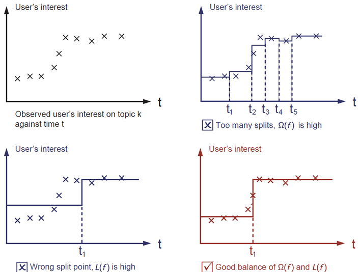
The correct answer is marked in red. Please consider if this visually seems a reasonable fit to you. The general principle is we want both a simple and predictive model. The tradeoff between the two is also referred as bias-variance tradeoff in machine learning.

正确答案用红色标记。
请考虑这在视觉上是否适合您。
一般原则是我们想要一个简单的预测模型。
两者之间的权衡在机器学习中也称为偏差-方差权衡。

Why introduce the general principle?

The elements introduced above form the basic elements of supervised learning, and they are natural building blocks of machine learning toolkits. For example, you should be able to describe the differences and commonalities between gradient boosted trees and random forests. Understanding the process in a formalized way also helps us to understand the objective that we are learning and the reason behind the heuristics such as pruning and smoothing.

为什么要介绍一般原则？

上面介绍的元素构成了监督学习的基本元素，
它们是机器学习工具包的天然构建块。
例如，您应该能够描述梯度提升树和随机森林之间的差异和共性。
以形式化的方式理解该过程还有助于我们理解
我们正在学习的目标以及启发式算法
（例如修剪和平滑）背后的原因。

Decision Tree Ensembles

Now that we have introduced the elements of supervised learning, let us get started with real trees. To begin with, let us first learn about the model choice of XGBoost: decision tree ensembles. The tree ensemble model consists of a set of classification and regression trees (CART). Here’s a simple example of a CART that classifies whether someone will like a hypothetical computer game X.

决策树集成

现在我们已经介绍了监督学习的元素，
让我们从真正的树开始。
首先，让我们先了解一下 XGBoost 的模型选择：决策树集成。
树集成模型由一组分类和回归树 (CART) 组成。
这是一个简单的 CART 示例，
用于对某人是否喜欢假设的计算机游戏 X 进行分类。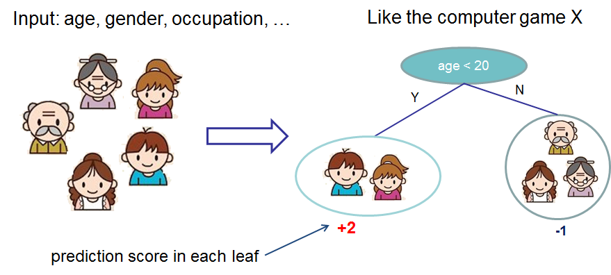

We classify the members of a family into different leaves, and assign them the score on the corresponding leaf. A CART is a bit different from decision trees, in which the leaf only contains decision values. In CART, a real score is associated with each of the leaves, which gives us richer interpretations that go beyond classification. This also allows for a principled, unified approach to optimization, as we will see in a later part of this tutorial.

我们将一个家庭的成员分为不同的叶子，
并在相应的叶子上为他们分配分数。
CART 与决策树有点不同，
决策树的叶子只包含决策值。
在 CART 中，真实分数与每个叶子相关联，
这为我们提供了超越分类的更丰富的解释。
这也允许有原则的、统一的优化方法，
我们将在本教程的后面部分看到。

Usually, a single tree is not strong enough to be used in practice. What is actually used is the ensemble model, which sums the prediction of multiple trees together.

通常，单个树的强度不足以在实践中使用。
实际使用的是ensemble模型，
将多棵树的预测汇总在一起。

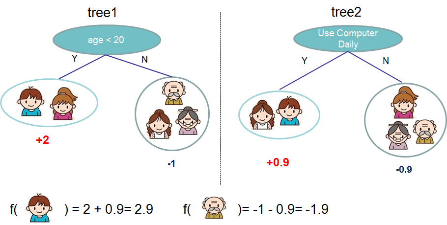
Here is an example of a tree ensemble of two trees. The prediction scores of each individual tree are summed up to get the final score. If you look at the example, an important fact is that the two trees try to complement each other. Mathematically, we can write our model in the form

这是一个由两棵树组成的树集合的例子。
每棵树的预测分数相加得到最终分数。
如果你看这个例子，一个重要的事实是两棵树试图相互补充。
在数学上，我们可以将我们的模型写成以下形式

其中 是树的数量，
是功能空间中的一个函数，
是所有可能的 CART 的集合。
要优化的目标函数由下式给出

Now here comes a trick question: what is the model used in random forests? Tree ensembles! So random forests and boosted trees are really the same models; the difference arises from how we train them. This means that, if you write a predictive service for tree ensembles, you only need to write one and it should work for both random forests and gradient boosted trees. (See Treelite for an actual example.) One example of why elements of supervised learning rock.

现在来一个棘手的问题：
随机森林中使用的模型是什么？
树木组合！
所以随机森林和提升树实际上是相同的模型；
区别在于我们如何训练他们。
这意味着，如果您为树集成编写预测服务，
您只需要编写一个，
它应该适用于随机森林和梯度提升树。
（有关实际示例，请参阅 Treelite。）
一个示例说明了监督学习的元素为何如此摇摆不定。

Tree Boosting

Now that we introduced the model, let us turn to training: How should we learn the trees? The answer is, as is always for all supervised learning models: define an objective function and optimize it!
Let the following be the objective function (remember it always needs to contain training loss and regularization):

树提升

现在我们介绍了模型，
让我们转向训练：
我们应该如何学习树？
答案是，
就像所有监督学习模型一样：
定义一个目标函数并对其进行优化！

让以下成为目标函数
（记住它总是需要包含训练损失和正则化）：

Additive Training

The first question we want to ask: what are the parameters of trees? You can find that what we need to learn are those functions fi, each containing the structure of the tree and the leaf scores. Learning tree structure is much harder than traditional optimization problem where you can simply take the gradient. It is intractable to learn all the trees at once. Instead, we use an additive strategy: fix what we have learned, and add one new tree at a time. We write the prediction value at step t as y^i(t). Then we have

附加训练
我们要问的第一个问题：树的参数是什么？
可以发现，我们需要学习的是那些函数，
每个函数都包含树的结构和叶子分数。
学习树结构比传统的优化问题要困难得多，
传统的优化问题可以简单地取梯度。
一次学习所有的树是很难的。
相反，我们使用了一种附加策略：
修复我们学到的东西，一次添加一棵树。
我们将步骤 t 的预测值写为 。 然后我们有

It remains to ask: which tree do we want at each step? A natural thing is to add the one that optimizes our objective.

剩下的问题是：
我们在每一步都想要哪棵树？
很自然的事情是添加优化我们的目标的那个。

If we consider using mean squared error (MSE) as our loss function, the objective becomes
如果我们考虑使用均方误差 (MSE) 作为我们的损失函数，
则目标变为：

The form of MSE is friendly, with a first order term (usually called the residual) and a quadratic term. For other losses of interest (for example, logistic loss), it is not so easy to get such a nice form. So in the general case, we take the Taylor expansion of the loss function up to the second order:

MSE的形式是友好的，
有一个一阶项（通常称为残差）和一个二次项。
对于其他的兴趣损失（例如，logistic loss），
要得到这么好的形式并不是那么容易。
所以在一般情况下，
我们将损失函数的泰勒展开式提升到二阶：

where the and are defined as
其中 和 定义为

After we remove all the constants, the specific objective at step becomes
在我们删除所有常量后，步骤 的特定目标变为

This becomes our optimization goal for the new tree. One important advantage of this definition is that the value of the objective function only depends on and . This is how XGBoost supports custom loss functions. We can optimize every loss function, including logistic regression and pairwise ranking, using exactly the same solver that takes and as input!

这成为我们对新树的优化目标。
该定义的一个重要优点是目标函数的值仅取决于 和 。
这就是 XGBoost 支持自定义损失函数的方式。
我们可以使用以 和作为输入的完全相同的求解器来优化每个损失函数，
包括逻辑回归和成对排名！