Hourly Time Series Forecasting using Facebook’s Prophet
基于Facebook的Prophet算法完成时间序列预测
项目URL:https://www.kaggle.com/robikscube/time-series-forecasting-with-prophet
算法具体参数设置:https://blog.csdn.net/wjskeepmaking/article/details/64905745
算法逻辑:https://blog.csdn.net/a358463121/article/details/70194279
底层算法逻辑:https://blog.csdn.net/weixin_39445556/article/details/84502260
基本模型
y(t)=g(t)+s(s)+h(t)+ϵt
这里,模型将时间序列分成3个部分的叠加,其中g(t)g(t)表示增长函数,用来拟合非周期性变化的。s(t)s(t)用来表示周期性变化,比如说每周,每年,季节等,h(t)h(t)表示假期,节日等特殊原因等造成的变化,最后ϵtϵt为噪声项,用他来表示随机无法预测的波动,我们假设ϵtϵt是高斯的。事实上,这是generalized additive model(GAM)模型的特例,但我们这里只用到了时间作为拟合的参数。
数据集:只有历史时间序列数据以及对应时间产生的用电量
| Datetime | PJME_MW |
|---|---|
| 2002-12-31 01:00:00 | 26498.0 |
| 2002-12-31 02:00:00 | 25147.0 |
| 2002-12-31 03:00:00 | 24574.0 |
| 2002-12-31 04:00:00 | 24393.0 |
| 2002-12-31 05:00:00 | 24860.0 |
# Setup and train model
model = Prophet()
model.fit(pjme_train.resetindex().rename(columns={‘Datetime’:’ds’,’PJME_MW’:’y’}))
#Predict on training set with model_
pjme_test_fcst = model.predict(df=pjme_test.reset_index().rename(columns={‘Datetime’:’ds’}))

随着预测时间的加长,预测精度的波动范围也逐渐扩大

趋势性,日期维度、周维度、月维度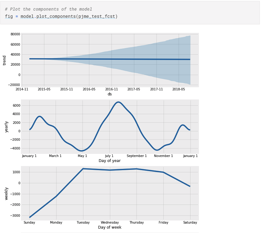
可以增加节假日特征来预测
Zillow Prize: Zillow’s Home Value Prediction (Zestimate)
房价预测
Kaggle URL:https://www.kaggle.com/sudalairajkumar/simple-exploration-notebook-zillow-prize
缺失值检查
missing_df = prop_df.isnull().sum(axis=0).reset_index()
missing_df.columns = [‘column_name’, ‘missing_count’]
missing_df = missing_df.ix[missing_df[‘missing_count’]>0]
missing_df = missing_df.sort_values(by=’missing_count’)
ind = np.arange(missing_df.shape[0])
width = 0.9
fig, ax = plt.subplots(figsize=(12,18))
rects = ax.barh(ind, missing_df.missing_count.values, color=’blue’)
ax.set_yticks(ind)
ax.set_yticklabels(missing_df.column_name.values, rotation=’horizontal’)
ax.set_xlabel(“Count of missing values”)
ax.set_title(“Number of missing values in each column”)
plt.show()

各特征和目标变量之间的相关性
# Now let us look at the correlation coefficient of each of these variables #
x_cols = [col for col in train_df_new.columns if col not in [‘logerror’] if train_df_new[col].dtype==’float64’]
labels = []
values = []
for col in xcols:
labels.append(col)
values.append(np.corrcoef(train_df_new[col].values, train_df_new.logerror.values)[0,1])
corr_df = pd.DataFrame({‘col_labels’:labels, ‘corr_values’:values})
corr_df = corr_df.sort_values(by=’corr_values’)
ind = np.arange(len(labels))
width = 0.9
fig, ax = plt.subplots(figsize=(12,40))
rects = ax.barh(ind, np.array(corr_df.corr_values.values), color=’y’)
ax.set_yticks(ind)
ax.set_yticklabels(corr_df.col_labels.values, rotation=’horizontal’)
ax.set_xlabel(“Correlation coefficient”)
ax.set_title(“Correlation coefficient of the variables”)
#autolabel(rects)_
plt.show()

若有收获,就点个赞吧
0 人点赞
