B树

本文翻译自 https://habr.com/en/company/postgrespro/blog/443284/，已经得作者同意。

我们已经讨论了 PostgreSQL 索引引擎和访问方法接口，以及其中一种访问方法：哈希索引。本文将介绍最传统且使用最广泛的索引：B-树。长文警告，请各位保持耐心。

B树

结构

B-树索引类型是 btree 访问方法的一种实现，适用于可排序的数据。也就是说，数据类型必须定义 greater , greator or equal , less , less or equal 和 equal 这些运算符。注意，相同的数据有时可能排序不同，这跟我们之前提到的运算符族的概念有关。

类似地，B-树的索引行也保存在对应的页中。叶子页（leaf page）中的索引行包含被索引的数据（key）和指向数据行的 TID；内部页（internal page）中，每行数据指向其一个孩子页，并且保存了该孩子页的最小值。

B-树有几个重要的特性：

B-树是平衡树，这意味着每个叶子与根之间有相同数量的内部页。即，搜索任何值的时间是相同的。
B-树是多路平衡树，即每个页（通常为 8KB）包含很多（数以百计）TID。因此，B-树的深度很小，对于非常大的表深度大概 4-5 层。
索引中的数据以非递减序（页面之间和页面内部都是）排列，同一层的页面通过双向链表彼此连接。因此，我们可以遍历链表或者反向遍历链表得到排序的数据，而无需每次都返回根页查找。

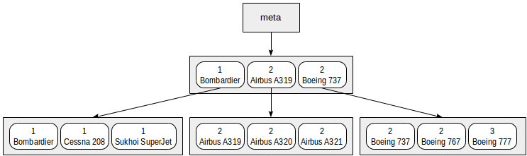
以下是一个简单的以整数为键的索引示例：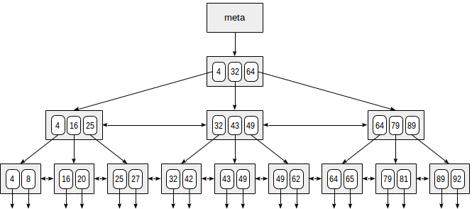

索引的第一个页是 mate 页，其指向索引的根节点。内部节点在根节点之下，叶子节点在最下层。最下边向下的箭头表示从叶子节点指向数据行（TID）。

等值搜索

我们来看看如何在树中通过一个形如 indexed-filed = expression 的等值条件搜索一个值。不妨假设我们想查询的键是 49。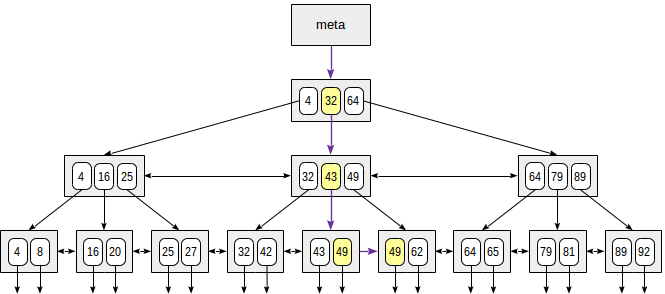

搜索从根节点开始，随后需要确定向下到哪个子节点继续搜索。由于知晓根节点的值是（4，32，64），我们可以计算出孩子节点中值的范围。由于 32 <= 49 < 64，我们需要到第二个孩子节点中搜索。接下来，重复递归相同的过程，直到到达叶子节点，从中获取到需要的 TID。

事实上，许多细节使这个看似简单的过程变得复杂。比如，索引键的值可能不是唯一的，且相同的值可能有很多，多到一个页都不足以容纳。还是回到上边的例子，也许在第二层查找时，我们应该定位到 49，但可以清楚地看到，这样将会跳过前一个叶子节点中的一个 49。因此，一旦在内部节点中找到一个与键值完全相等的值，我们必须向左挪动一个位置，然后从左到右查看其下层的索引行，以搜索所需的键。

（另一个复杂的问题是，在搜索期间，其他进程有可能会修复数据：树可能被重建，页面可能分裂等等。工程上所有算法都是为这些并发操作而设计的，确保这些操作不会相互干扰，也不会导致额外的锁开销。本文将尽量避免在这方面进行展开。）

非等值搜索

当使用形如 indexed-filed <= expression 的条件搜索时，首先通过等值条件 indexed-filed = expression 在索引中找到一个匹配的值（如果有的话），然后沿适当的方向遍历叶子节点直到结束。

下图描述了按条件 n <= 35 搜索的过程：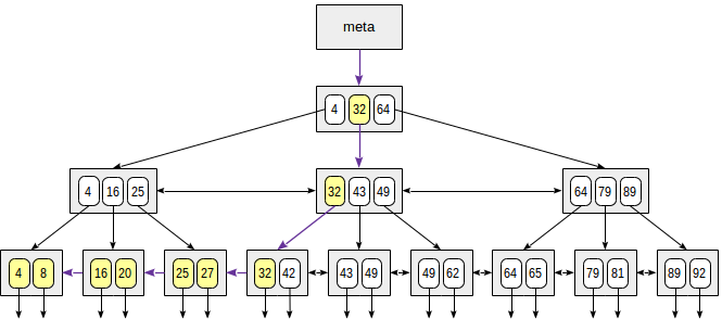

greater 和 less 运算符的搜索过程是类似的，但必须删除最初找到的相等的值。

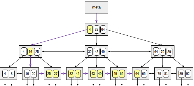
范围搜索

当使用形如 expression1 <= indexed-field <= expression2 的范围条件搜索时，我们通过条件 indexed-field == expression1 找到一个值，然后遍历叶子节点，直到不再满足 indexed-field <= expression2 的条件；或者相反的顺序，从第二个表达式开始，然后沿相反的方向遍历叶子节点，直到不再满足第一个表达式。

下图描述了按条件 23 <= n <= 64 搜索的过程：

举例

我们来看一个使用 B-树的查询计划示例。照例使用我们的演示数据库，这次使用 aircrafts 表，仅包含 9 行数据。由于整张表仅有一页数据，计划器不会选择使用索引。但这个表在满足我们说明目的的同时还比较有趣，因此选择它。

demo=# select * from aircrafts;
 aircraft_code |        model        | range 
---------------+---------------------+-------
 773           | Boeing 777-300      | 11100
 763           | Boeing 767-300      |  7900
 SU9           | Sukhoi SuperJet-100 |  3000
 320           | Airbus A320-200     |  5700
 321           | Airbus A321-200     |  5600
 319           | Airbus A319-100     |  6700
 733           | Boeing 737-300      |  4200
 CN1           | Cessna 208 Caravan  |  1200
 CR2           | Bombardier CRJ-200  |  2700
(9 rows)
demo=# create index on aircrafts(range);
demo=# set enable_seqscan = off;

（或者显式地用 using btree(range) 在 aircrafts 表上创建索引，若不指定，默认创建的就是 B-树索引。）

等值搜索：

demo=# explain(costs off) select * from aircrafts where range = 3000;
                    QUERY PLAN                     
---------------------------------------------------
 Index Scan using aircrafts_range_idx on aircrafts
   Index Cond: (range = 3000)
(2 rows)

不等式搜索：

demo=# explain(costs off) select * from aircrafts where range < 3000;
QUERY PLAN                    
---------------------------------------------------
 Index Scan using aircrafts_range_idx on aircrafts
   Index Cond: (range < 3000) 
(2 rows)

范围搜索：

demo=# explain(costs off) select * from aircrafts
where range between 3000 and 5000;
                     QUERY PLAN                      
-----------------------------------------------------
 Index Scan using aircrafts_range_idx on aircrafts
   Index Cond: ((range >= 3000) AND (range <= 5000))
(2 rows)

排序

再次强调，无论使用何种扫描方式（index，index-only 或 bitmap）， btree 访问方法都返回有序的数据，从上文的图示中也可以清楚地看到这一点。

因此，如果一个表在排序条件上有索引，优化器将有两种选择：索引扫描，或顺序扫描并对结果排序。

排列顺序

创建索引时可以显式指定排列顺序，比如，我们可以按航班飞行距离创建索引：

demo=# create index on aircrafts(range desc);

此时，较大的值将在 B 树的左侧，而较小的值在右侧。既然我们可以从两个方向上遍历索引值，为什么还需要指定排列顺序呢？

其目的是多列索引。我们创建一个视图，将飞机划分为短程、中程和远程：

demo=# create view aircrafts_v as
select model,
       case
           when range < 4000 then 1
           when range < 10000 then 2
           else 3
       end as class
from aircrafts;
demo=# select * from aircrafts_v;
       model        | class
---------------------+-------
 Boeing 777-300      |     3
 Boeing 767-300      |     2
 Sukhoi SuperJet-100 |     1
 Airbus A320-200     |     2
 Airbus A321-200     |     2
 Airbus A319-100     |     2
 Boeing 737-300      |     2
 Cessna 208 Caravan  |     1
 Bombardier CRJ-200  |     1
(9 rows)

然后，创建一个表达式索引：

demo=# create index on aircrafts(
  (case when range < 4000 then 1 when range < 10000 then 2 else 3 end),
  model);

现在，我们可以使用索引来获取按两列升序排列的数据。

demo=# select class, model from aircrafts_v order by class, model;
 class |        model        
-------+---------------------
     1 | Bombardier CRJ-200
     1 | Cessna 208 Caravan
     1 | Sukhoi SuperJet-100
     2 | Airbus A319-100
     2 | Airbus A320-200
     2 | Airbus A321-200
     2 | Boeing 737-300
     2 | Boeing 767-300
     3 | Boeing 777-300
(9 rows)
demo=# explain(costs off)
select class, model from aircrafts_v order by class, model;
                       QUERY PLAN                       
--------------------------------------------------------
 Index Scan using aircrafts_case_model_idx on aircrafts
(1 row)

同样，也可以获取降序排列的数据：

demo=# select class, model from aircrafts_v order by class desc, model desc;
 class |        model        
-------+---------------------
     3 | Boeing 777-300
     2 | Boeing 767-300
     2 | Boeing 737-300
     2 | Airbus A321-200
     2 | Airbus A320-200
     2 | Airbus A319-100
     1 | Sukhoi SuperJet-100
     1 | Cessna 208 Caravan
     1 | Bombardier CRJ-200
(9 rows)
demo=# explain(costs off)
select class, model from aircrafts_v order by class desc, model desc;
                           QUERY PLAN                            
-----------------------------------------------------------------
 Index Scan BACKWARD using aircrafts_case_model_idx on aircrafts
(1 row)

然而，我们无法使用该索引获取按一列降序、另一列升序的数据。这需要额外的排序操作：

demo=# explain(costs off)
select class, model from aircrafts_v order by class ASC, model DESC;
                   QUERY PLAN                    
-------------------------------------------------
 Sort
   Sort Key: (CASE ... END), aircrafts.model DESC
   ->  Seq Scan on aircrafts
(3 rows)

（注意，计划器无视我们上文中设置的 enable_seqscan=off 仍然选择了顺序扫描。事实上，这种设置并不能禁止表扫描，而只是将扫描代价设置为较大的值。可以在执行 explian 时设置 cost on 来查看代价。）

为了使该查询可以使用索引，需要创建一个满足所需排序的索引：

demo=# create index aircrafts_case_asc_model_desc_idx on aircrafts(
 (case
    when range < 4000 then 1
    when range < 10000 then 2
    else 3
  end) ASC,
  model DESC);
demo=# explain(costs off)
select class, model from aircrafts_v order by class ASC, model DESC;
                           QUERY PLAN                            
-----------------------------------------------------------------
 Index Scan using aircrafts_case_asc_model_desc_idx on aircrafts
(1 row)

列的顺序

使用多列索引时的另一个问题是索引中列的顺序。对于 B-树索引而言，顺序是非常重要的：页面内的数据首先按第一个字段排序，然而按第二个字段排序，以此类推。

我们可以用下图表示在 range 和 model 上创建的多列索引：

事实上，一个根节点足以容纳这样一个很小的索引。但为方便描述，上图特意将其分布在多个页中。

从上图可以清楚地看到，通过诸如 class = 3 （仅通过第一个字段进行搜索）或 class = 3 and model = 'Boeing 777-300' (同时搜索两个字段) 这样的谓词搜索将会非常高效。

而根据谓词 model = 'Boeing 777-300' 进行搜索的效率则很低：从根节点开始，我们无法判断应该向下搜索哪个子节点，因此必须搜索每一个子节点。但这并不意味着这样的索引不能使用，只是效率堪忧。例如，如果我们有三类飞机，每一类又有很多型号，我们将不得不扫描整个索引的约 1/3，这可能比全表扫描更加高效，当然，也可能相反。

如果我们创建如下索引：

demo=# create index on aircrafts(
  model,
  (case when range < 4000 then 1 when range < 10000 then 2 else 3 end));

字段的排序将会发生改变：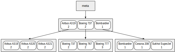

创建该索引之后，通过谓词 model = 'Boeing 777-300' 搜索将非常高效，而通过谓词 class = 3 搜索的效率则不尽如人意。

NULL

btree 访问方法可以索引 NULL 值，并支持通过 IS NULL 和 IS NOT NULL 进行搜索。

让我们看看有 NULL 值得 flights 表：

demo=# create index on flights(actual_arrival);
demo=# explain(costs off) select * from flights where actual_arrival is null;
                      QUERY PLAN                       
-------------------------------------------------------
 Bitmap Heap Scan on flights
   Recheck Cond: (actual_arrival IS NULL)
   ->  Bitmap Index Scan on flights_actual_arrival_idx
         Index Cond: (actual_arrival IS NULL)
(4 rows)

NULL 值位于叶子节点的一端或者另一端的末尾，具体取决于创建索引的方法（NULLS FIRST 或 NULLS LAST）。这对包含排序的查询是至关重要的：如果 SELECT 命令在其 ORDER BY 子句中指定的 NULL 值顺序与创建索引时指定的 NULL 值顺序相同（NULLS FIRST 或 NULLS LAST），则可以使用该索引。

以下例子中，查询要求的 NULL 值排序就与索引的 NULL 值排序相同，因此可以使用索引：

demo=# explain(costs off)
select * from flights order by actual_arrival NULLS LAST;
                       QUERY PLAN                      
--------------------------------------------------------
 Index Scan using flights_actual_arrival_idx on flights
(1 row)

以下查询要求的 NULL 值排序则与索引不同，因此，优化器选择顺序扫描并进行排序：

demo=# explain(costs off)
select * from flights order by actual_arrival NULLS FIRST;
               QUERY PLAN              
----------------------------------------
 Sort
   Sort Key: actual_arrival NULLS FIRST
   ->  Seq Scan on flights
(3 rows)

该查询若想使用索引，需要创建一个 NULL 值排在前面的索引：

demo=# create index flights_nulls_first_idx on flights(actual_arrival NULLS FIRST);
demo=# explain(costs off)
select * from flights order by actual_arrival NULLS FIRST;
                     QUERY PLAN                      
-----------------------------------------------------
 Index Scan using flights_nulls_first_idx on flights
(1 row)

NULL 值只能存储在所有叶子节点最开始或最末尾这个问题的根本原因是 NULL 值不能进行排序，即 NULL 与其他任何值比较的结果都是未定义的。

demo=# \pset null NULL
demo=# select null < 42;
 ?column?
----------
 NULL
(1 row)

这与 B-树的概念背道而驰，也区别于一般的模式。而 NULL 在数据库系统中扮演着非常重要的角色，因此我们不得不为它做一些特殊处理。

由于 NULL 可以被索引，使得即便没有在表上施加任何条件也可以使用索引成为可能（因为索引肯定包含表中所有行的信息，包括是 NULL 的行）。如果查询需要排序，并且索引可以确保所需的顺序，那么这可能是有意义的。在这种情况下，计划器可以选择索引访问避免一次额外的排序操作。

属性

我们来看 btree 访问方法的属性（查询方法在之前的文章中已经给出）.

 amname |     name      | pg_indexam_has_property
--------+---------------+-------------------------
 btree  | can_order     | t
 btree  | can_unique    | t
 btree  | can_multi_col | t
 btree  | can_exclude   | t

如上所示，B-树可以对数据进行排序，并支持唯一索引—这是唯一一个支持类似属性的访问方法。B-树也支持多列索引，当然也有其他访问方法（尽管不是全部）支持多列索引。支持 EXCLUDE 约束也有其原因，我们后续会讨论。

  name      | pg_index_has_property
---------------+-----------------------
 clusterable   | t
 index_scan    | t
 bitmap_scan   | t
 backward_scan | t

bree 访问方法支持两种扫描方式：index scan 和 bitmap scan。如上所示，也支持正向（ forword）和反向（ backward）对树进行遍历。

 name        | pg_index_column_has_property 
--------------------+------------------------------
 asc                | t
 desc               | f
 nulls_first        | f
 nulls_last         | t
 orderable          | t
 distance_orderable | f
 returnable         | t
 search_array       | t
 search_nulls       | t

前四个属性说明特定列的值是如何被排序的。本例中，值按照递增（ asc）和 NULL 在最后（ null_las ）的方式排序。当然，如上文所说，其他组合也是有可能的。

search_array 属性说明支持如下表达式使用索引：

demo=# explain(costs off)
select * from aircrafts where aircraft_code in ('733','763','773');
                           QUERY PLAN                            
-----------------------------------------------------------------
 Index Scan using aircrafts_pkey on aircrafts
   Index Cond: (aircraft_code = ANY ('{733,763,773}'::bpchar[]))
(2 rows)

returnable 属性说明支持 index-only scan，这是合理的，因为索引行本身存储了被索引的值（与哈希索引不同）。这里有必要谈一谈基于 B-树的覆盖索引。

具有附加行的唯一索引

如之前文章所述，覆盖索引存储了查询所需的所有数据，（几乎）不需要再访问数据表本身。

假设为满足查询所需，我们想为唯一索引增加一个额外的列。但这种组合值的唯一性不能保证原先唯一索引键的唯一性，因此，需要在同一个列上建两个索引：一个唯一索引支持完整性约束，另一个用于覆盖。显然这是比较低效的。

我的同事 Anastasiya Lubennikova 改进了 btree 方法，使 btree 索引可以包含附件的、非唯一的列。该特性在 PostgreSQL 11 中已经支持了。

我们来看 bookings 表：

demo=# \d bookings
              Table "bookings.bookings"
    Column    |           Type           | Modifiers
--------------+--------------------------+-----------
 book_ref     | character(6)             | not null
 book_date    | timestamp with time zone | not null
 total_amount | numeric(10,2)            | not null
Indexes:
    "bookings_pkey" PRIMARY KEY, btree (book_ref)
Referenced by:
    TABLE "tickets" CONSTRAINT "tickets_book_ref_fkey" FOREIGN KEY (book_ref) REFERENCES bookings(book_ref)

该表中，主键 (book_ref) 是一个普通的 btree 索引。我们创建一个带有附加列的唯一索引：

demo=# create unique index bookings_pkey2 on bookings(book_ref) INCLUDE (book_date);

现在，我们用这个新索引替换之前的旧索引（在事务中，同时应用所有的变化）：

demo=# begin;
demo=# alter table bookings drop constraint bookings_pkey cascade;
demo=# alter table bookings add primary key using index bookings_pkey2;
demo=# alter table tickets add foreign key (book_ref) references bookings (book_ref);
demo=# commit;

结果如下：

demo=# \d bookings
              Table "bookings.bookings"
    Column    |           Type           | Modifiers
--------------+--------------------------+-----------
 book_ref     | character(6)             | not null
 book_date    | timestamp with time zone | not null
 total_amount | numeric(10,2)            | not null
Indexes:
    "bookings_pkey2" PRIMARY KEY, btree (book_ref) INCLUDE (book_date)
Referenced by:
    TABLE "tickets" CONSTRAINT "tickets_book_ref_fkey" FOREIGN KEY (book_ref) REFERENCES bookings(book_ref)

现在，同一个索引既满足唯一约束，又可以用于覆盖索引，如下：

demo=# explain(costs off)
select book_ref, book_date from bookings where book_ref = '059FC4';
                    QUERY PLAN                    
--------------------------------------------------
 Index Only Scan using bookings_pkey2 on bookings
   Index Cond: (book_ref = '059FC4'::bpchar)
(2 rows)

索引的创建

众所周知，对于非常大的表，加载数据时最好不带索引，数据导入之后再创建所需的索引。这样不仅速度更快，而且索引可能更小。

其原因在于，创建 btree 索引会使用一种比按行插入更加高效的方式。大体而言，表中所有数据先排好序，并创建这些数据对应的叶子节点，然后基于这些叶子节点创建内部节点，直到整个金字塔收敛到根节点。

这个构建过程的速度取决于可使用内存的大小，由参数 maintenance_work_mem 决定，增加该参数的值，可以加快处理速度。对于唯一索引，除 maintenance_work_mem 之外，还需要分配 work_mem 大小的内存。

比较语义

介绍哈希索引时我们提到，PostgreSQL 需要知道不同数据类型的值应该使用哪个哈希函数，这种对应关系存储在 hash 访问方法中。同样，系统也必须知道如何对值进行排序。这在排序、分组（有时）、归并连接等操作中是必需的。PostgreSQL … TODO：

例如，这些比较运算符用于 bool_ops 运算符族：

postgres=# select   amop.amopopr::regoperator as opfamily_operator,
         amop.amopstrategy
from     pg_am am,
         pg_opfamily opf,
         pg_amop amop
where    opf.opfmethod = am.oid
and      amop.amopfamily = opf.oid
and      am.amname = 'btree'
and      opf.opfname = 'bool_ops'
order by amopstrategy;
  opfamily_operator  | amopstrategy
---------------------+-------------- 
 <(boolean,boolean)  |            1
 <=(boolean,boolean) |            2
 =(boolean,boolean)  |            3
 >=(boolean,boolean) |            4
 >(boolean,boolean)  |            5
(5 rows)

这里，我们看到五个比较运算符，但正如前文提到的，我们不应该依赖他们的名字。为了搞清楚每个运算符都做哪些比较，引入了策略（strategy）的概念。定义了五种策略来描述运算符的语义：

1 — less
2 — less or equal
3 — equal
4 — greater or equal
5 — greater

一些运算符族可以包含实现一个策略的多个运算符。例如， integer_ops 运算符族包含以下策略为 1 的运算符：

postgres=# select   amop.amopopr::regoperator as opfamily_operator
from     pg_am am,
         pg_opfamily opf,
         pg_amop amop
where    opf.opfmethod = am.oid
and      amop.amopfamily = opf.oid
and      am.amname = 'btree'
and      opf.opfname = 'integer_ops'
and      amop.amopstrategy = 1
order by opfamily_operator;
  opfamily_operator  
---------------------- 
 <(integer,bigint)
 <(smallint,smallint)
 <(integer,integer)
 <(bigint,bigint)
 <(bigint,integer)
 <(smallint,integer)
 <(integer,smallint)
 <(smallint,bigint)
 <(bigint,smallint)
(9 rows)

由于这些特性，优化器在比较一个运算符族中包含的不同类型的值时，可以不用做类型转换。

索引支持新数据类型

官方文档中有一个创建新数据类型的例子：复数以及对其值排序的运算符类。这个例子是用 C 语言写的，如果考虑执行效率，用 C 语言写当然无可厚非。但为了更好地理解“比较”的语义，我们用 SQL 来做一个同样的实验。

创建一个包含两个字段的新复合类型：实部和虚部。

postgres=# create type complex as (re float, im float);

建一张使用新类型的表，并添加一些值：

postgres=# create table numbers(x complex);
postgres=# insert into numbers values ((0.0, 10.0)), ((1.0, 3.0)), ((1.0, 1.0));

问题来了，如果没有在数学意义上为复数定义顺序关系，如何对它们进行排序？

事实证明，比较运算符已经定义好了。

postgres=# select * from numbers order by x;
   x    
--------
 (0,10)
 (1,1)
 (1,3)
(3 rows)

默认情况下，对于复合类型，排序是按照组合字段进行的：首先比较第一个字段，然后比较第二个字段，以此类推。这与逐个字符比较字符串类似。但我们可以定义不同的排序。例如，可以将复数看做向量，按模（长度）排序，模（长度）等于直角坐标中平方和的平方根（毕达哥拉斯定理）。为了定义这样的顺序，我们创建一个计算模的辅助函数：

postgres=# create function modulus(a complex) returns float as $$
    select sqrt(a.re*a.re + a.im*a.im);
$$ immutable language sql;

现在，使用此辅助函数为所有 5 个比较运算符定义对应的比较函数：

postgres=# create function complex_lt(a complex, b complex) returns boolean as $$
    select modulus(a) < modulus(b);
$$ immutable language sql;
postgres=# create function complex_le(a complex, b complex) returns boolean as $$
    select modulus(a) <= modulus(b);
$$ immutable language sql;
postgres=# create function complex_eq(a complex, b complex) returns boolean as $$
    select modulus(a) = modulus(b);
$$ immutable language sql;
postgres=# create function complex_ge(a complex, b complex) returns boolean as $$
    select modulus(a) >= modulus(b);
$$ immutable language sql;
postgres=# create function complex_gt(a complex, b complex) returns boolean as $$
    select modulus(a) > modulus(b);
$$ immutable language sql;

创建对应的运算符。为了说明运算符无需命名为 “>”，”<” 等，我们给它们起一些怪异的名字。

postgres=# create operator #<#(leftarg=complex, rightarg=complex, procedure=complex_lt);
postgres=# create operator #<=#(leftarg=complex, rightarg=complex, procedure=complex_le);
postgres=# create operator #=#(leftarg=complex, rightarg=complex, procedure=complex_eq);
postgres=# create operator #>=#(leftarg=complex, rightarg=complex, procedure=complex_ge);
postgres=# create operator #>#(leftarg=complex, rightarg=complex, procedure=complex_gt);

现在，我们可以比较复数了：

postgres=# select (1.0,1.0)::complex #<# (1.0,3.0)::complex;
 ?column?
----------
 t
(1 row)

除以上 5 个运算符， btree 访问方法还需要定义一个额外的函数：第一个值小于、等于或大于第二个值时，分别返回-1，0 或 1。这个辅助函数称为 support 函数。其他访问方法可能需要定义其他的 support 函数。

postgres=# create function complex_cmp(a complex, b complex) returns integer as $$
    select case when modulus(a) < modulus(b) then -1
                when modulus(a) > modulus(b) then 1 
                else 0
           end;
$$ language sql;

现在，我们创建一个运算符类（与此同时会自动创建一个同名的运算符族）：

postgres=# create operator class complex_ops
default for type complex
using btree as
    operator 1 #<#,
    operator 2 #<=#,
    operator 3 #=#,
    operator 4 #>=#,
    operator 5 #>#,
    function 1 complex_cmp(complex,complex);

现在就可以根据我们的需要排序了：

postgres=# select * from numbers order by x;
   x    
--------
 (1,1)
 (1,3)
 (0,10)
(3 rows)

以上，btree 就支持我们新定义的数据类型了。可以使用以下查询获取 support 函数：

postgres=# select amp.amprocnum,
       amp.amproc,
       amp.amproclefttype::regtype,
       amp.amprocrighttype::regtype
from   pg_opfamily opf,
       pg_am am,
       pg_amproc amp
where  opf.opfname = 'complex_ops'
and    opf.opfmethod = am.oid
and    am.amname = 'btree'
and    amp.amprocfamily = opf.oid;
 amprocnum |   amproc    | amproclefttype | amprocrighttype
-----------+-------------+----------------+-----------------
         1 | complex_cmp | complex        | complex
(1 row)

内部结构

我们可以使用 pageinspect 插件一探 B-树内部的结构。

demo=# create extension pageinspect;

索引 meta 页：

demo=# select * from bt_metap('ticket_flights_pkey');
 magic  | version | root | level | fastroot | fastlevel
--------+---------+------+-------+----------+-----------
 340322 |       2 |  164 |     2 |      164 |         2
(1 row)

这里最有趣的是索引层数（level）：一个包含一百万行数据的表，在两个列上创建索引，仅仅有两层（不包括根节点）。

块 164（root）的统计信息如下：

demo=# select type, live_items, dead_items, avg_item_size, page_size, free_size
from bt_page_stats('ticket_flights_pkey',164);
 type | live_items | dead_items | avg_item_size | page_size | free_size
------+------------+------------+---------------+-----------+-----------
 r    |         33 |          0 |            31 |      8192 |      6984
(1 row)

块中的数据内容如下（ data 以二进制形式表示索引的键值）：

demo=# select itemoffset, ctid, itemlen, left(data,56) as data
from bt_page_items('ticket_flights_pkey',164) limit 5;
 itemoffset |  ctid   | itemlen |                           data                           
------------+---------+---------+----------------------------------------------------------
          1 | (3,1)   |       8 |
          2 | (163,1) |      32 | 1d 30 30 30 35 34 33 32 33 30 35 37 37 31 00 00 ff 5f 00
          3 | (323,1) |      32 | 1d 30 30 30 35 34 33 32 34 32 33 36 36 32 00 00 4f 78 00
          4 | (482,1) |      32 | 1d 30 30 30 35 34 33 32 35 33 30 38 39 33 00 00 4d 1e 00
          5 | (641,1) |      32 | 1d 30 30 30 35 34 33 32 36 35 35 37 38 35 00 00 2b 09 00
(5 rows)

真正的索引元组数据从第二个字段开始， ctid 记录其子节点的信息。显然，最左侧的子节点是块 163，随后是 323，以此类推。同样可以使用相同的函数来探究其他块的内容。其他字段的含义大家可以阅读官方文档，README 和源码，在此不多加阐述。

PostgreSQL 从 10 版本开始支持了 amcheck 模块，可以检测 B-树中数据的逻辑一致性，使我们能够提前检测故障。

PostgreSQL必知必会

PostgreSQL 索引-4.B树

B树

结构