本章概要

本章讲述线性模型（linear model），相关内容包括：

• 线性回归（linear regression）

  序关系（order）、均方差（square error）最小化、欧式距离（Euclidean distance）、最小二乘法（least square method）、参数估计（parameter estimation）、多元线性回归（multivariate linear regression）、广义线性回归（generalized linear model）、对数线性回归（log-linear regression）；

• 对数几率回归（逻辑回归）（logistic regression）

  分类、Sigmoid函数、对数几率（log odds / logit）、极大似然法（maximum likelihood method）；

• 线性判别分析（linear discriminant analysis - LDA）

  类内散度（within-class scatter）、类间散度（between-class scatter）；

• 多分类学习（multi-classifier）

  拆解法，一对一（One vs One - OvO）、一对其余（OvR）、多对多（MvM）、纠错输出码（ECOC）、编码矩阵（coding matrix）、二元码、多标记学习（multi-label learning）；

• 类别不平衡（class-imbalance）

  再缩放（rescaling）、欠采样（undersampling）、过采样（oversampling）、阈值移动（threshold-moving）；

习题解答

3.1 线性回归模型偏置项

偏置项b在数值上代表了自变量取0时，因变量的取值；
1.当讨论变量x对结果y的影响，不用考虑b；
2.可以用变量归一化（max-min或z-score）来消除偏置。

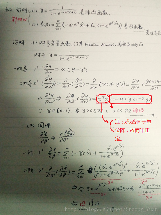
3.2 证明对数似然函数是凸函数（参数存在最优解）

直接给出证明结果如下图：

3.3 编程实现对率回归

所使用的数据集如下：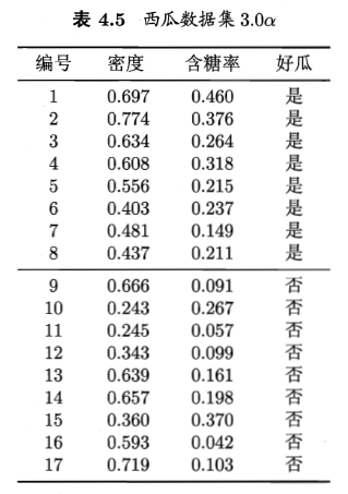

   首先，我们要构造跃阶函数，也就是sigmoid函数，书中给的函数是:<br />![](https://cdn.nlark.com/yuque/0/2020/png/1061864/1594789906137-ae24183b-c0ca-4cf0-8185-d610809f31d7.png#align=left&display=inline&height=41&margin=%5Bobject%20Object%5D&originHeight=41&originWidth=94&size=0&status=done&style=none&width=94)<br />由这个跃阶函数来处理二分类问题。

但是，这个跃阶函数的效果不是太好，亲自试验过，发现效果不是一般的差。一般都是用

这个公式来计算，也就是上图注释掉的代码。

import numpy as np
import matplotlib.pyplot as plt


def sigmoid(inX):
    # return 1.0/(1+np.exp(-inX))
    return 2*1.0/(1+np.exp(-2*inX))-1


# 训练
def gradAscend(data,labels):
    m = data.shape[0]         # 行
    n = data.shape[1]         # 列
    step = 0.001
    time = 1000
    wights = np.ones((n,1))
    for i in range(time):
        h = sigmoid(data*wights)
        error = labels-h
        wights = wights+step*data.T*error
    return wights


def createDataSet():
    group = np.matrix([[0.697,0.460,1],
                       [0.774,0.376,1],
                       [0.634,0.264,1],
                       [0.608,0.318,1],
                       [0.556,0.215,1],
                       [0.403,0.237,1],
                       [0.481,0.149,1],
                       [0.437,0.211,1],
                       [0.666,0.091,1],
                       [0.243,0.267,1],
                       [0.245,0.057,1],
                       [0.343,0.099,1],
                       [0.639,0.161,1],
                       [0.657,0.198,1],
                       [0.360,0.370,1],
                       [0.593,0.042,1],
                       [0.719,0.103,1]])
    labels = np.matrix([[1],[1],[1],[1],[1],[1],[1],[1],[0],[0],[0],[0],[0],[0],[0],[0],[0]])
    return group, labels


group, labels = createDataSet()
w = gradAscend(group,labels)
data = np.array(group)
X1 = []
Y1 = []
X2 = []
Y2 = []
for i in range(7):
    X1.append(data[i,0])
    Y1.append(data[i,1])
for i in range(7,16):
    X2.append(data[i,0])
    Y2.append(data[i,1])
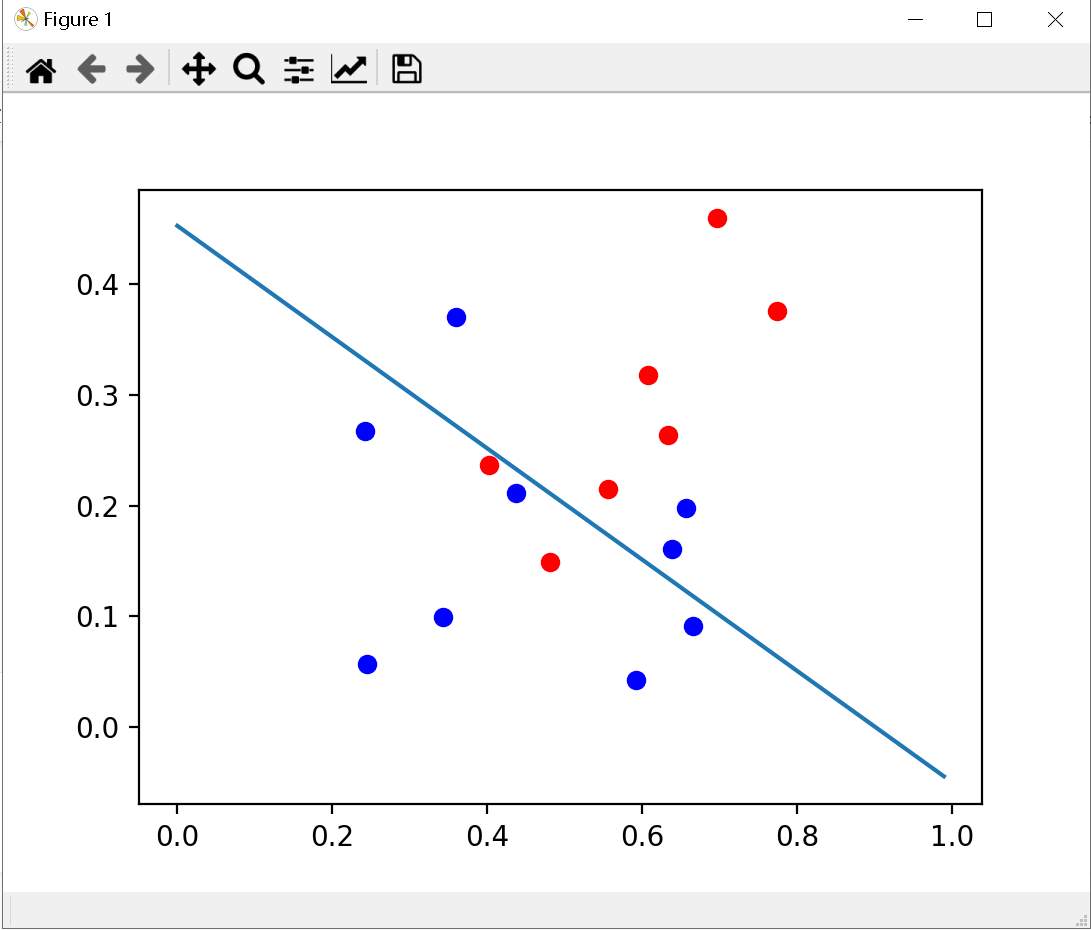
plt.scatter(X1, Y1, c='red')
plt.scatter(X2, Y2, c='blue')
x1 = np.arange(0, 1, step=0.01)
plt.plot(x1, (0.5 - x1 * w[0,0] - w[2,0]) / w[1,0])
plt.show()
print(w)

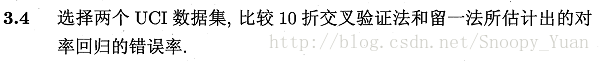
3.4 比较k折交叉验证法与留一法

本题采用UCI中的 Iris Data Set 和 Blood Transfusion Service Center Data Set，基于sklearn完成练习。

关于数据集的介绍：
IRIS数据集简介 - 百度百科；通过花朵的性状数据（花萼大小、花瓣大小…）来推测花卉的类别。变量属性X=4种，类别标签y公有3种，这里我们选取其中两类数据来拟合对率回归(逻辑斯蒂回归)。

Blood Transfusion Service Center Data Set - UCI;通过献血行为（上次献血时间、总献血cc量…）的历史数据，来推测某人是否会在某一时段献血。变量属性X=4种，类别y={0,1}。该数据集相对iris要大一些。

具体过程如下：

1. 数据导入、可视化、预分析：

iris数据集十分常用，sklearn的数据包已包含该数据集，我们可以直接载入，也可以下载后导入。对于transfusion数据集，我们从UCI官网上下载导入即可。
采用seaborn库可以实现基于matplotlib的非常漂亮的可视化呈现效果，下图是采用seaborn.pairplot()绘制的iris数据集各变量关系组合图，从图中可以看出，类别区分十分明显，分类器应该比较容易实现：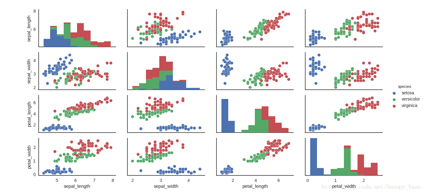

相关样例代码：

import numpy as np
import seaborn as sns
sns.set(style="white", color_codes=True)
iris = sns.load_dataset("iris")

iris.plot(kind="scatter", x="sepal_length", y="sepal_width")
sns.pairplot(iris,hue='species') 
sns.plt.show()

2. 基于sklearn进行拟合与交叉验证：

这里我们选择iris中的两类数据对应的样本进行分析。k-折交叉验证可直接根据sklearn.model_selection.cross_val_predict()得到精度、F1值等度量（该函数要求1＜k＜n-1）。留一法稍微复杂一点，这里采用loop实现。

面向iris数据集的样例代码：

import numpy as np
import seaborn as sns
from sklearn.linear_model import LogisticRegression
from sklearn import metrics
from sklearn.model_selection import cross_val_predict, LeaveOneOut

sns.set(style="white", color_codes=True)
iris = sns.load_dataset("iris")
X = iris.values[50:150, 0:4]
y = iris.values[50:150, 4]

iris.plot(kind="scatter", x="sepal_length", y="sepal_width")
sns.pairplot(iris, hue='species')
sns.plt.show()


# 2-nd logistic regression using sklearn

# log-regression lib model
log_model = LogisticRegression()
m = np.shape(X)[0]

# 10-folds CV
y_pred = cross_val_predict(log_model, X, y, cv=10)
print(metrics.accuracy_score(y, y_pred))

# LOOCV
from sklearn.model_selection import LeaveOneOut

loo = LeaveOneOut()
accuracy = 0
for train, test in loo.split(X):
    log_model.fit(X[train], y[train])  # fitting
    y_p = log_model.predict(X[test])
    if y_p == y[test]: accuracy += 1
print(accuracy / np.shape(X)[0])

得出了精度（预测准确度）结果如下：

0.97
0.96

可以看到，两种方法的模型精度都十分高，这也得益于iris数据集类间散度较大。

面向transfusion数据集的样例代码

from sklearn.linear_model import LogisticRegression
from sklearn import metrics
from sklearn.model_selection import cross_val_predict, LeaveOneOut
import numpy as np

dataset_transfusion = np.loadtxt('transfusion.data', delimiter=",", skiprows=1)
X2 = dataset_transfusion[:, 0:4]
y2 = dataset_transfusion[:, 4]

# log-regression lib model
log_model = LogisticRegression()
m = np.shape(X2)[0]

# 10-folds CV
y2_pred = cross_val_predict(log_model, X2, y2, cv=10)
print(metrics.accuracy_score(y2, y2_pred))

# LOOCV
loo = LeaveOneOut()
accuracy = 0;
for train, test in loo.split(X2):
    log_model.fit(X2[train], y2[train])  # fitting
    y2_p = log_model.predict(X2[test])
    if y2_p == y2[test]: accuracy += 1
print(accuracy / np.shape(X2)[0])

结果：

0.76
0.77

也可以看到，两种交叉验证的结果相近，但是由于此数据集的类分性不如iris明显，所得结果也要差一些。同时由程序运行可以看出，LOOCV的运行时间相对较长，这一点随着数据量的增大而愈发明显。

所以，一般情况下选择K-折交叉验证即可满足精度要求，同时运算量相对小。