Clair是7岁还是8岁

Predict["NameAge", "Claire"]

8

distribution = Predict["NameAge", "Claire", "Distribution"]

dataRaw = distribution[[2]]

{{0.0436854,0.0434454,0.0417851,0.0410707,0.039174,0.0392846,0.0341221,0.0297407,0.0301554,0.0321928,0.0306963,0.0328238,0.0335628,0.0337617,0.0329839,0.0274761,0.0247628,0.0226914,0.0199307,0.0174267,0.0178853,0.016748,0.0156118,0.0142017,0.0121872,0.0112472,0.0110289,0.0101354,0.0083158,0.00727845,0.00693834,0.00579045,0.00500136,0.00476404,0.00422787,0.0042015,0.00330494,0.00382356,0.00353463,0.00397766,0.00267746,0.0029375,0.00324305,0.00358885,0.00338324,0.00364493,0.00472906,0.00431149,0.00502461,0.005541,0.00667215,0.00666396,0.00624235,0.00699836,0.00670012,0.00723419,0.006929,0.00514928,0.00543192,0.0056786,0.00566318,0.00556554,0.00404206,0.00422927,0.00398858,0.00459221,0.00433242,0.00287366,0.00315304,0.00314997,0.00326664,0.00302409,0.00243289,0.00236613,0.00272464,0.00246009,0.00277903,0.0011675,0.00135807,0.00141423,0.00155165,0.00169708,0.00113741,0.00117819,0.00120093,0.00127315,0.00115479,0.000524236,0.00055232,0.000490803,0.000470074,0.000428617},{7,8,9,10,11,12,13,14,15,16,17,18,19,20,21,22,23,24,25,26,27,28,29,30,31,32,33,34,35,36,37,38,39,40,41,42,43,44,45,46,47,48,49,50,51,52,53,54,55,56,57,58,59,60,61,62,63,64,65,66,67,68,69,70,71,72,73,74,75,76,77,78,79,80,81,82,83,84,85,86,87,88,89,90,91,92,93,94,95,96,97,98,99}}

Length /@ dataRaw

{92,93}

Let’s see this distribution, this is not the paired data. Functions like HistogramDistribution receives paired data.

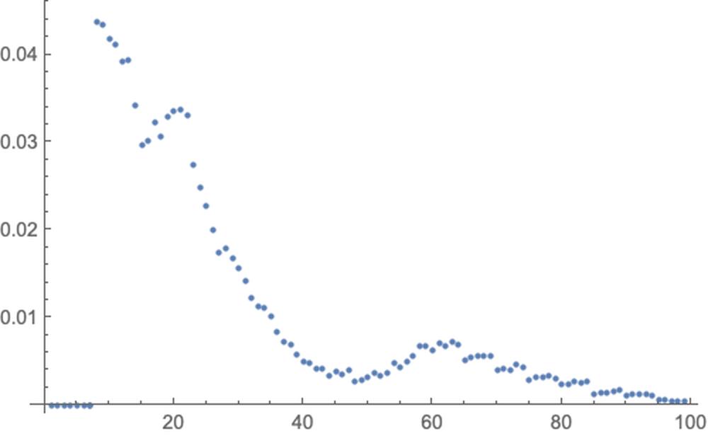
If we pad data in the Left, we can do like the following, we can ListPlot the data.

data = Reverse /@ Transpose@{ConstantArray[0, 8]~Join~#[[1]], Range[1, 7]~Join~#[[2]]} &@distribution[[2]]

{{1,0},{2,0},{3,0},{4,0},{5,0},{6,0},{7,0},{7,0},{8,0.0436854},{9,0.0434454},{10,0.0417851},{11,0.0410707},{12,0.039174},{13,0.0392846},{14,0.0341221},{15,0.0297407},{16,0.0301554},{17,0.0321928},{18,0.0306963},{19,0.0328238},{20,0.0335628},{21,0.0337617},{22,0.0329839},{23,0.0274761},{24,0.0247628},{25,0.0226914},{26,0.0199307},{27,0.0174267},{28,0.0178853},{29,0.016748},{30,0.0156118},{31,0.0142017},{32,0.0121872},{33,0.0112472},{34,0.0110289},{35,0.0101354},{36,0.0083158},{37,0.00727845},{38,0.00693834},{39,0.00579045},{40,0.00500136},{41,0.00476404},{42,0.00422787},{43,0.0042015},{44,0.00330494},{45,0.00382356},{46,0.00353463},{47,0.00397766},{48,0.00267746},{49,0.0029375},{50,0.00324305},{51,0.00358885},{52,0.00338324},{53,0.00364493},{54,0.00472906},{55,0.00431149},{56,0.00502461},{57,0.005541},{58,0.00667215},{59,0.00666396},{60,0.00624235},{61,0.00699836},{62,0.00670012},{63,0.00723419},{64,0.006929},{65,0.00514928},{66,0.00543192},{67,0.0056786},{68,0.00566318},{69,0.00556554},{70,0.00404206},{71,0.00422927},{72,0.00398858},{73,0.00459221},{74,0.00433242},{75,0.00287366},{76,0.00315304},{77,0.00314997},{78,0.00326664},{79,0.00302409},{80,0.00243289},{81,0.00236613},{82,0.00272464},{83,0.00246009},{84,0.00277903},{85,0.0011675},{86,0.00135807},{87,0.00141423},{88,0.00155165},{89,0.00169708},{90,0.00113741},{91,0.00117819},{92,0.00120093},{93,0.00127315},{94,0.00115479},{95,0.000524236},{96,0.00055232},{97,0.000490803},{98,0.000470074},{99,0.000428617}}

data // Length

100

ListPlot@data

If we use PDF to extract data, we can see there is a zero in the end of list.

pdf[x_] := PDF[distribution, x]
list = Table[pdf[x], {x, 0, 99}]

{0,0,0,0,0,0,0,0.0436854,0.0434454,0.0417851,0.0410707,0.039174,0.0392846,0.0341221,0.0297407,0.0301554,0.0321928,0.0306963,0.0328238,0.0335628,0.0337617,0.0329839,0.0274761,0.0247628,0.0226914,0.0199307,0.0174267,0.0178853,0.016748,0.0156118,0.0142017,0.0121872,0.0112472,0.0110289,0.0101354,0.0083158,0.00727845,0.00693834,0.00579045,0.00500136,0.00476404,0.00422787,0.0042015,0.00330494,0.00382356,0.00353463,0.00397766,0.00267746,0.0029375,0.00324305,0.00358885,0.00338324,0.00364493,0.00472906,0.00431149,0.00502461,0.005541,0.00667215,0.00666396,0.00624235,0.00699836,0.00670012,0.00723419,0.006929,0.00514928,0.00543192,0.0056786,0.00566318,0.00556554,0.00404206,0.00422927,0.00398858,0.00459221,0.00433242,0.00287366,0.00315304,0.00314997,0.00326664,0.00302409,0.00243289,0.00236613,0.00272464,0.00246009,0.00277903,0.0011675,0.00135807,0.00141423,0.00155165,0.00169708,0.00113741,0.00117819,0.00120093,0.00127315,0.00115479,0.000524236,0.00055232,0.000490803,0.000470074,0.000428617,0}

list // Length

100

My question 1 is why there is a 0 in the end of the list
My question2 is why there is no 0 values in dataRaw, and why the data in zero is not paired data.

How to make this example not so confused.

My question3 is: The max value of data of years is 8 or 7?
The data from real world, the most frequent year maybe 7, but in the learned model, it becomes 8, 8 is the 8th position.
Is it a bug of the model? If we maximize the pdf function, we can get 7.

Maximize[pdf[x], x]

{0.0436854,{x->7.01018}}

<< "/Users/hypergroups/Nutstore/Wolfram \Mathematica/DeployProjects/MyMarkDown/MyMarkDown.wl"
Notebook2Markdown[EvaluationNotebook[],  "dirOutput" -> NotebookDirectory[], "title" -> "year_of_Clair",  ImagePrefix -> "https://raw.githubusercontent.com/HyperGroups/Mathematica/master/\YuQue/mathematica/MachineLearningInAction/year_of_Clair"]