一、理论知识及其原理
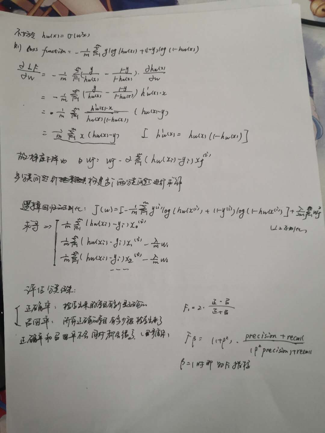
关于原理,可以参照https://blog.csdn.net/u011734144/article/details/79717470和笔记即可
笔记截图:
二、线性逻辑回归
1.梯度下降法的应用
import matplotlib.pyplot as pltimport numpy as npfrom sklearn.metrics import classification_reportfrom sklearn import preprocessing# 数据是否需要标准化scale = False# 载入数据data = np.genfromtxt(r"C:\Users\小新\Desktop\课程pdf\py\机器学习\逻辑回归\LR-testSet.csv", delimiter=",")x_data = data[:,:-1] #切分除了最后一列的数据都是xy_data = data[:,-1] #切分最后一列为y,这里的y_data是分类类别(取值0和1)def plot(): #定义这个函数是用来画出下面的图的x0 = [] #分类类别对应的值x1 = [] #分类类别对应的值y0 = [] #分类类别为0y1 = [] #分类类别为1# 切分不同类别的数据for i in range(len(x_data)): #数据切分if y_data[i] == 0: #说明这是第0个类别x0.append(x_data[i,0]) #存放第0个特征y0.append(x_data[i,1]) #存放第1个特征else:x1.append(x_data[i,0])y1.append(x_data[i,1])# 画图scatter0 = plt.scatter(x0, y0, c='b', marker='o') #0类别的散点图scatter1 = plt.scatter(x1, y1, c='r', marker='x') #1类别的散点图#画图例plt.legend(handles=[scatter0,scatter1],labels=['label0','label1'],loc='best') #loc是选择最佳位置plot()plt.show()#注:这里可以用以下代码快速画图:x_data = data[:,:-1]y_data = data[:,-1]plt.scatter(x.data[:,0],x_data[:,1],color = y_data) #直接利用y_data来进行颜色赋值(y_data本来是二分类变量)plt.show()# 数据处理,添加偏置项x_data = data[:,:-1]y_data = data[:,-1,np.newaxis] #增加维度print(np.mat(x_data).shape) #100行2列print(np.mat(y_data).shape) #100行1列(相当于列向量)# 给样本添加偏置项X_data = np.concatenate((np.ones((100,1)),x_data),axis=1)print(X_data.shape) #100行3列#开始进行逻辑回归def sigmoid(x): #定义sigmoid函数return 1.0/(1+np.exp(-x))def cost(xMat, yMat, ws): #定义损失函数,xmat是训练数据,ymat是标签,ws是权值(都是矩阵形式)left = np.multiply(yMat, np.log(sigmoid(xMat*ws))) #损失函数左边的部分,np.multiply是对应位置元素相乘,yMat和np.log(sigmoid(xMat*ws)都是100*1的right = np.multiply(1 - yMat, np.log(1 - sigmoid(xMat*ws))) #损失函数的右边部分return np.sum(left + right) / -(len(xMat)) #得到最终的损失函数#注:这里损失函数用矩阵乘法会不会成功?可以试试看def gradAscent(xArr, yArr):if scale == True:xArr = preprocessing.scale(xArr) #对数据进行标准化xMat = np.mat(xArr)yMat = np.mat(yArr)lr = 0.001 #定义学习率epochs = 10000 #定义迭代次数costList = [] #保存cost值,每次迭代都会产生一个新的cost# 计算数据行列数# 行代表数据个数,列代表权值个数m,n = np.shape(xMat) #m代表行,n代表列# 初始化权值ws = np.mat(np.ones((n,1))) #都初始化为1for i in range(epochs+1):# xMat和weights矩阵相乘h = sigmoid(xMat*ws) #损失函数中hθ(x),100行1列# 计算误差ws_grad = xMat.T*(h - yMat)/m #计算梯度,矩阵乘法,3行100列乘以100行1列,得到3行1列,即系数值,公式中的求和项相当于在矩阵里进行了ws = ws - lr*ws_gradif i % 50 == 0:costList.append(cost(xMat,yMat,ws)) #每隔50次保存一次cost值return ws,costList#注:#1,2#3,4#4,3#2,1#得到矩阵为##4,6##6,4# 训练模型,得到权值和cost值的变化ws,costList = gradAscent(X_data, y_data)print(ws)if scale == False: #非标准化的数据,标准化后的数据数值改变后画图会很奇怪,于是标准化后的图可以不用画# 画图决策边界plot()x_test = [[-4],[3]] #规定x的取值y_test = (-ws[0] - x_test*ws[1])/ws[2] #这里令w0+xw1+yw2 = 0(sigmoid分界点→0.5)求解y(边界)plt.plot(x_test, y_test, 'k')plt.show()# 画图 loss值的变化x = np.linspace(0,10000,201) #从0到10000画200个点plt.plot(x, costList, c='r')plt.title('Train')plt.xlabel('Epochs')plt.ylabel('Cost')plt.show()# 预测def predict(x_data, ws):if scale == True:x_data = preprocessing.scale(x_data)xMat = np.mat(x_data)ws = np.mat(ws)return [1 if x >= 0.5 else 0 for x in sigmoid(xMat*ws)] #如果x大于等于0.5,返回类别1,小于0.5,返回类别0predictions = predict(X_data, ws)print(classification_report(y_data, predictions)) #正确率,召回率的查看情况
2.sklearn库的方法
import matplotlib.pyplot as pltimport numpy as npfrom sklearn.metrics import classification_reportfrom sklearn import preprocessingfrom sklearn import linear_model# 数据是否需要标准化scale = False# 载入数据data = np.genfromtxt(r"C:\Users\小新\Desktop\课程pdf\py\机器学习\逻辑回归\LR-testSet.csv", delimiter=",")x_data = data[:,:-1]y_data = data[:,-1]def plot():x0 = []x1 = []y0 = []y1 = []# 切分不同类别的数据for i in range(len(x_data)):if y_data[i]==0:x0.append(x_data[i,0])y0.append(x_data[i,1])else:x1.append(x_data[i,0])y1.append(x_data[i,1])# 画图scatter0 = plt.scatter(x0, y0, c='b', marker='o')scatter1 = plt.scatter(x1, y1, c='r', marker='x')#画图例plt.legend(handles=[scatter0,scatter1],labels=['label0','label1'],loc='best')plot()plt.show()logistic = linear_model.LogisticRegression() #利用sklearn库进行逻辑回归logistic.fit(x_data, y_data)#其余相关的参数如截距、回归系数的代码跟回归分析类似,在这里不过多赘述if scale == False:# 画图决策边界,注意这里是二维的,多维的情况不宜画图plot()x_test = np.array([[-4],[3]])y_test = (-logistic.intercept_ - x_test*logistic.coef_[0][0])/logistic.coef_[0][1] #logistic.coef_是一个1*2的矩阵形式,这里的[0]是取第一行的两个数,转化成一个向量形式,第二个[0],[1]就是取这两个数了plt.plot(x_test, y_test, 'k')plt.show()predictions = logistic.predict(x_data)print(classification_report(y_data, predictions)) #计算正确率、召回率和F1值
三、非线性逻辑回归
1.梯度下降法的应用
import matplotlib.pyplot as pltimport numpy as npfrom sklearn.metrics import classification_reportfrom sklearn import preprocessingfrom sklearn.preprocessing import PolynomialFeatures# 数据是否需要标准化scale = False# 载入数据data = np.genfromtxt(r"C:\Users\小新\Desktop\课程pdf\py\机器学习\逻辑回归\LR-testSet2.txt", delimiter=",")x_data = data[:,:-1]y_data = data[:,-1,np.newaxis]def plot():x0 = []x1 = []y0 = []y1 = []# 切分不同类别的数据for i in range(len(x_data)):if y_data[i]==0:x0.append(x_data[i,0])y0.append(x_data[i,1])else:x1.append(x_data[i,0])y1.append(x_data[i,1])# 画图scatter0 = plt.scatter(x0, y0, c='b', marker='o')scatter1 = plt.scatter(x1, y1, c='r', marker='x')#画图例plt.legend(handles=[scatter0,scatter1],labels=['label0','label1'],loc='best')plot()plt.show()# 定义多项式回归,degree的值可以调节多项式的特征,自己可以多次尝试poly_reg = PolynomialFeatures(degree=3) #做数据多项式处理# 特征处理x_poly = poly_reg.fit_transform(x_data)##注:特征处理我们来举个例子:##test = [[2,3]]# 定义多项式回归,degree的值可以调节多项式的特征#poly_reg = PolynomialFeatures(degree=3)# 特征处理#x_poly = poly_reg.fit_transform(test) #构造出非线性项,包括交互项#x_poly #这里给出的第一个是x的偏置项,第二第三个是x1,x2,第四个是x1^2,第五个是x1*x2,第六个是x2^2,第七个是x2^3,第八个是x1^2*x2,第九个是x1*x2^2,第十个是x2^3#output情况:array([[ 1., 2., 3., 4., 6., 9., 8., 12., 18., 27.]])def sigmoid(x):return 1.0/(1+np.exp(-x))def cost(xMat, yMat, ws):left = np.multiply(yMat, np.log(sigmoid(xMat*ws)))right = np.multiply(1 - yMat, np.log(1 - sigmoid(xMat*ws)))return np.sum(left + right) / -(len(xMat))def gradAscent(xArr, yArr):if scale == True:xArr = preprocessing.scale(xArr)xMat = np.mat(xArr)yMat = np.mat(yArr)lr = 0.03epochs = 50000costList = []# 计算数据列数,有几列就有几个权值m,n = np.shape(xMat)# 初始化权值ws = np.mat(np.ones((n,1)))for i in range(epochs+1):# xMat和weights矩阵相乘h = sigmoid(xMat*ws)# 计算误差ws_grad = xMat.T*(h - yMat)/mws = ws - lr*ws_gradif i % 50 == 0:costList.append(cost(xMat,yMat,ws))return ws,costList# 训练模型,得到权值和cost值的变化ws,costList = gradAscent(x_poly, y_data)print(ws)#画决策边界情况(手操较难)# 获取数据值所在的范围【决定数据下图数据框的大小】x_min, x_max = x_data[:, 0].min() - 1, x_data[:, 0].max() + 1y_min, y_max = x_data[:, 1].min() - 1, x_data[:, 1].max() + 1# 生成网格矩阵xx, yy = np.meshgrid(np.arange(x_min, x_max, 0.02),np.arange(y_min, y_max, 0.02))# np.r_按row来组合array,# np.c_按colunm来组合array# >>> a = np.array([1,2,3])# >>> b = np.array([5,2,5])# >>> np.r_[a,b]# array([1, 2, 3, 5, 2, 5])# >>> np.c_[a,b]# array([[1, 5],# [2, 2],# [3, 5]])# >>> np.c_[a,[0,0,0],b]# array([[1, 0, 5],# [2, 0, 2],# [3, 0, 5]])z = sigmoid(poly_reg.fit_transform(np.c_[xx.ravel(), yy.ravel()]).dot(np.array(ws)))# ravel与flatten类似,多维数据转一维(使之扁平化)。flatten不会改变原始数据,ravel会改变原始数据#z函数相当于把网格矩阵的点给做一个预测,是1就是一类,是0就是一类,利用密集点填充的方式来强行构造出一个边界for i in range(len(z)):if z[i] > 0.5:z[i] = 1else:z[i] = 0z = z.reshape(xx.shape)# 等高线图cs = plt.contourf(xx, yy, z)plot()plt.show()# 预测def predict(x_data, ws):# if scale == True:# x_data = preprocessing.scale(x_data)xMat = np.mat(x_data)ws = np.mat(ws)return [1 if x >= 0.5 else 0 for x in sigmoid(xMat*ws)]predictions = predict(x_poly, ws)print(classification_report(y_data, predictions))
2.sklearn库的方法
import numpy as npimport matplotlib.pyplot as pltfrom sklearn import linear_modelfrom sklearn.datasets import make_gaussian_quantilesfrom sklearn.preprocessing import PolynomialFeatures# 生成2维正态分布,生成的数据按分位数分为两类,500个样本,2个样本特征# 可以生成两类或多类数据x_data, y_data = make_gaussian_quantiles(n_samples=500, n_features=2,n_classes=2)plt.scatter(x_data[:, 0], x_data[:, 1], c=y_data)plt.show()logistic = linear_model.LogisticRegression()logistic.fit(x_data, y_data)# 定义多项式回归,degree的值可以调节多项式的特征poly_reg = PolynomialFeatures(degree=5)# 特征处理x_poly = poly_reg.fit_transform(x_data)# 定义逻辑回归模型logistic = linear_model.LogisticRegression()# 训练模型logistic.fit(x_poly, y_data) #不指定x值会出现线性分类情况,所以需要自己去定义多项式部分!注意!# 获取数据值所在的范围x_min, x_max = x_data[:, 0].min() - 1, x_data[:, 0].max() + 1y_min, y_max = x_data[:, 1].min() - 1, x_data[:, 1].max() + 1# 生成网格矩阵xx, yy = np.meshgrid(np.arange(x_min, x_max, 0.02),np.arange(y_min, y_max, 0.02))# np.r_按row来组合array,# np.c_按colunm来组合array# >>> a = np.array([1,2,3])# >>> b = np.array([5,2,5])# >>> np.r_[a,b]# array([1, 2, 3, 5, 2, 5])# >>> np.c_[a,b]# array([[1, 5],# [2, 2],# [3, 5]])# >>> np.c_[a,[0,0,0],b]# array([[1, 0, 5],# [2, 0, 2],# [3, 0, 5]])z = logistic.predict(poly_reg.fit_transform(np.c_[xx.ravel(), yy.ravel()]))# ravel与flatten类似,多维数据转一维。flatten不会改变原始数据,ravel会改变原始数据z = z.reshape(xx.shape)# 等高线图cs = plt.contourf(xx, yy, z)# 样本散点图plt.scatter(x_data[:, 0], x_data[:, 1], c=y_data)plt.show()print('score:',logistic.score(x_poly,y_data)) #输出R方值

若有收获,就点个赞吧
0 人点赞


