Partial Dependency Plots

Partial Dependency Plots

Partial Dependency Plots（后续用PDP或PD简称）会展示一个或两个特征对于模型预测的边际效益（J. H. Friedman 2001）。PDP可以展示一个特征是如何影响预测的。与此同时，我们可以通过绘制特征和预测目标之间的一维关系图或二维关系图来了解特征与目标之间的关系。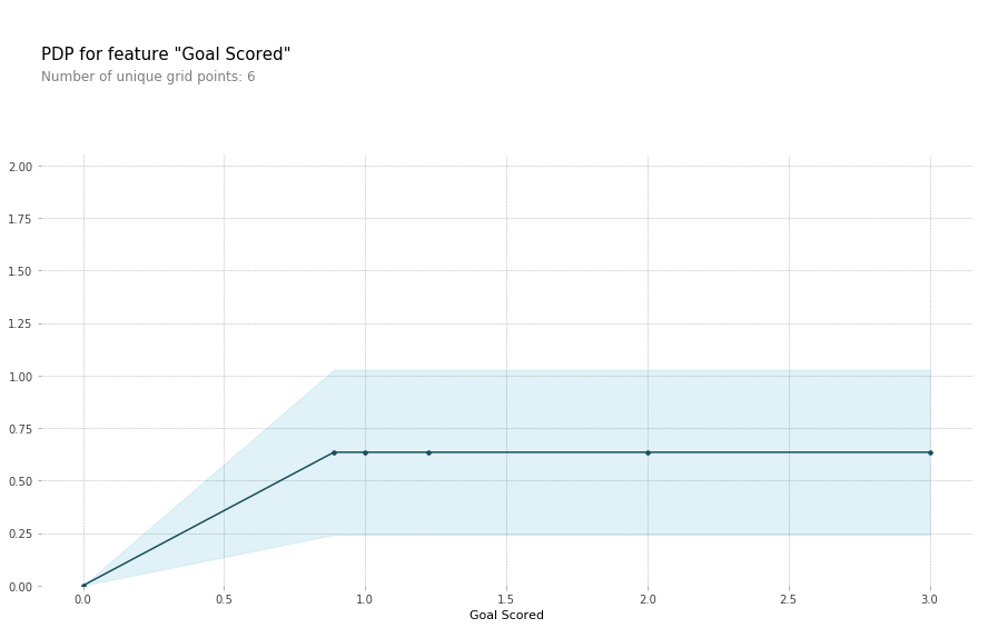

Do the shapes match your expectations for what shapes they would have? Can you explain the shape now that you’ve seen them?

Solution:
The code is

We have a sense from the permutation importance results that distance is the most important determinant of taxi fare.
This model didn’t include distance measures (like absolute change in latitude or longitude) as features, so coordinate features (like pickup_longitude) capture the effect of distance.
Being picked up near the center of the longitude values lowers predicted fares on average, because it means shorter trips (on average).

For the same reason, we see the general U-shape in all our partial dependence plots.

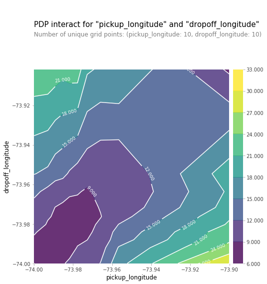
2D Plot

Create a 2D plot for the features pickup_longitude and dropoff_longitude. Plot it appropriately?
What do you expect it to look like?

Solution:
You should expect the plot to have contours running along a diagonal. We see that to some extent, though there are interesting caveats.
We expect the diagonal contours because these are pairs of values where the pickup and dropoff longitudes are nearby, indicating shorter trips (controlling for other factors).
As you get further from the central diagonal, we should expect prices to increase as the distances between the pickup and dropoff longitudes also increase.
The surprising feature is that prices increase as you go further to the upper-right of this graph, even staying near that 45-degree line.
This could be worth further investigation, though the effect of moving to the upper right of this graph is small compared to moving away from that 45-degree line.

The code you need to create the desired plot is:

fnames = ['pickup_longitude', 'dropoff_longitude']
longitudes_partial_plot  =  pdp.pdp_interact(
    model=first_model, dataset=val_X,
    model_features=base_features, 
    features=fnames
)
pdp.pdp_interact_plot(
    pdp_interact_out=longitudes_partial_plot,
    feature_names=fnames, plot_type='contour')
plt.show()

Question 04

Hint:
use the abs function when creating the abs_lat_change and abs_lon_change features.
You don’t need to change anything else.

# This is the PDP for pickup_longitude without the absolute difference features. Included here to help compare it to the new PDP you create
feat_name = 'pickup_longitude'
pdp_dist_original = pdp.pdp_isolate(model=first_model, dataset=val_X, model_features=base_features, feature=feat_name)
pdp.pdp_plot(pdp_dist_original, feat_name)
plt.show()

Solution:
The biggest difference is that the partial dependence plot became much smaller.
The the lowest vertical value is about 15 𝑏𝑒𝑙𝑜𝑤 𝑡ℎ𝑒 ℎ𝑖𝑔ℎ𝑒𝑠𝑡 𝑣𝑒𝑟𝑡𝑖𝑐𝑎𝑙 𝑣𝑎𝑙𝑢𝑒 𝑖𝑛 𝑡ℎ𝑒 𝑡𝑜𝑝 𝑐ℎ𝑎𝑟𝑡, 𝑤ℎ𝑒𝑟𝑒𝑎𝑠 𝑡ℎ𝑖𝑠 𝑑𝑖𝑓𝑓𝑒𝑟𝑒𝑛𝑐𝑒 𝑖𝑠 𝑜𝑛𝑙𝑦 𝑎𝑏𝑜𝑢𝑡 3 in the chart you just created.
In other words, once you control for absolute distance traveled, the pickup_longitude has only a very small impact on predictions.

# create new features
data['abs_lon_change'] = abs(data.dropoff_longitude - data.pickup_longitude)
data['abs_lat_change'] = abs(data.dropoff_latitude - data.pickup_latitude)

# create new features
data['abs_lon_change'] = ____
data['abs_lat_change'] = ____
features_2  = ['pickup_longitude',
               'pickup_latitude',
               'dropoff_longitude',
               'dropoff_latitude',
               'abs_lat_change',
               'abs_lon_change']
X = data[features_2]
new_train_X, new_val_X, new_train_y, new_val_y = train_test_split(X, y, random_state=1)
second_model = RandomForestRegressor(n_estimators=30, random_state=1).fit(new_train_X, new_train_y)
feat_name = 'pickup_longitude'
pdp_dist = pdp.pdp_isolate(model=second_model, dataset=new_val_X, model_features=features_2, feature=feat_name)
pdp.pdp_plot(pdp_dist, feat_name)
plt.show()

Question 05

Consider a scenario where you have only 2 predictive features, which we will call feat_A and feat_B. Both features have minimum values of -1 and maximum values of 1. The partial dependence plot for feat_A increases steeply over its whole range, whereas the partial dependence plot for feature B increases at a slower rate (less steeply) over its whole range.
Does this guarantee that feat_A will have a higher permutation importance than feat_B. Why or why not?

Solution:
No. This doesn’t guarantee feat_a is more important. For example, feat_a could have a big effect in the cases where it varies, but could have a single value 99% of the time.
In that case, permuting feat_a wouldn’t matter much, since most values would be unchanged.

Question 06

The code cell below does the following:

1. Creates two features, X1 and X2, having random values in the range [-2, 2].
2. Creates a target variable y, which is always 1.
3. Trains a RandomForestRegressor model to predict y given X1 and X2.
4. Creates a PDP plot for X1 and a scatter plot of X1 vs. y.

Do you have a prediction about what the PDP plot will look like? Run the cell to find out.
Modify the initialization of y so that our PDP plot has a positive slope in the range [-1,1], and a negative slope everywhere else. (Note: you should only modify the creation of y, leaving X1, X2, and my_model unchanged.)

import numpy as np
from numpy.random import rand
n_samples = 20000
# Create array holding predictive feature
X1 = 4 * rand(n_samples) - 2
X2 = 4 * rand(n_samples) - 2
# Create y. you should have X1 and X2 in the expression for y
y = -2 * X1 * (X1 < -1) + X1 -2 * X1* (X1>1) - X2
# create dataframe because pdp_isolate expects a dataFrame as an argument
my_df = pd.DataFrame({
    'X1': X1,
    'X2': X2,
    'y': y
})
predictors_df = my_df.drop(['y'], axis = 1)
my_model = RandomForestRegressor(
    n_estimators = 30,
    random_state = 1).fit(predictors_df, my_df.y)
pdp_dist = pdp.pdp_isolate(
    model = my_model,
    dataset = my_df,
    model_features = ['X1','X2'],
    feature = 'X1'
)
# visualize your results
pdp.pdp_plot(pdp_dist, 'X1')
plt.show()
# Check your answer
q_6.check()

Hint:
Consider explicitly using terms that include mathematical expressions like (X1 < -1)

Solution:

# There are many possible solutions.
# One example expression for y is.
y = -2 * X1 * (X1<-1) + X1 - 2 * X1 * (X1>1) - X2
# You don't need any more changes

Question 07

Create a dataset with 2 features and a target, such that the pdp of the first feature is flat, but its permutation importance is high.
We will use a RandomForest for the model.
Note:
You only need to supply the lines that create the variables X1, X2 and y. The code to build the model and calculate insights is provided.

Hints:
You need for X1 to affect the prediction in order to have it affect permutation importance. But the average effect needs to be 0 to satisfy the PDP requirement. Achieve this by creating an interaction, so the effect of X1 depends on the value of X2 and vice-versa.