Data From SHIYANLOU 實驗樓
01 Renthop 公司數據集
# 下载数据并解压!wget -nc "https://labfile.oss.aliyuncs.com/courses/1283/renthop_train.json.gz"!gunzip "renthop_train.json.gz"
02 Telecom Churn data 電信商
!wget 'https://labfile.oss.aliyuncs.com/courses/1283/telecom_churn.csv'
03 House Price 房價數據
!wget 'https://labfile.oss.aliyuncs.com/courses/1363/HousePrice.csv'
04 Titanic Data
!wget 'https://labfile.oss.aliyuncs.com/courses/1363/Titanic.csv'
05 SOCR Dataset
Weights and Heights
!wget 'https://labfile.oss.aliyuncs.com/courses/1283/weights_heights.csv' # 导入数据集
06 Adult Data
!wget 'https://labfile.oss.aliyuncs.com/courses/1283/adult.data.csv'data['salary'] = pd.factorize(data['salary'])[0]string = ['workclass', 'education', 'marital-status', 'relationship','occupation', 'race', 'sex']for i in string:data[i] = pd.factorize(data[i])[0]data.info()
07 Home Credit
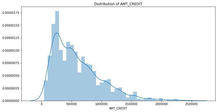
# Download data!wget "https://labfile.oss.aliyuncs.com/courses/1363/HomeCredit.csv"!ls# Import libraryimport pandas as pdimport matplotlib.pyplot as pltimport seaborn as snsimport warningswarnings.filterwarnings("ignore")%matplotlib inlinepath = 'HomeCredit.csv'house = pd.read_csv(path)house.head()# Main columnscolumn = ['AMT_CREDIT', 'AMT_INCOME_TOTAL', 'AMT_GOODS_PRICE','NAME_TYPE_SUITE', 'TARGET','NAME_CONTRACT_TYPE', 'NAME_INCOME_TYPE','NAME_FAMILY_STATUS','OCCUPATION_TYPE','NAME_EDUCATION_TYPE','NAME_HOUSING_TYPE','DAYS_BIRTH','DAYS_EMPLOYED']MainHouse = house[column]MainHouse.head()# Label Encodingfrom sklearn.preprocessing import LabelEncodercat_features = ['NAME_TYPE_SUITE', 'NAME_CONTRACT_TYPE', 'NAME_INCOME_TYPE','NAME_FAMILY_STATUS', 'OCCUPATION_TYPE','NAME_HOUSING_TYPE', 'NAME_EDUCATION_TYPE']for col in cat_features:encoder = LabelEncoder()value = list(MainHouse[col].values.astype('str'))encoder.fit(value)MainHouse[col] = encoder.transform(value)MainHouse.head()
The data preparation until the MainHouse data is generated.
08 Google Play
!wget -nc "https://labfile.oss.aliyuncs.com/courses/1363/googleplaystore.csv"!ls
LightGBM Encoding
import lightgbm as lgbfeature_cols = train.columns.drop('TARGET')dtrain = lgb.Dataset(train[feature_cols], label = train['TARGET'])dvalid = lgb.Dataset(train[feature_cols], label = valid['TARGET'])param = {'num_leaves': 64,'objective': "binary"}param['metric'] = 'auc'num_round = 1000bst = lgb.train(param, dtrain, num_round, valid_sets = [dvalid],early_stopping_rounds = 10,verbose_eval = False)
Example of Kaggle - Click
def train_model(train, valid, test=None, feature_cols=None):if feature_cols is None:feature_cols = train.columns.drop(['click_time', 'attributed_time','is_attributed'])dtrain = lgb.Dataset(train[feature_cols], label=train['is_attributed'])dvalid = lgb.Dataset(valid[feature_cols], label=valid['is_attributed'])param = {'num_leaves': 64, 'objective': 'binary','metric': 'auc', 'seed': 7}num_round = 1000print("Training model!")bst = lgb.train(param, dtrain, num_round, valid_sets=[dvalid],early_stopping_rounds=20, verbose_eval=False)valid_pred = bst.predict(valid[feature_cols])valid_score = metrics.roc_auc_score(valid['is_attributed'], valid_pred)print(f"Validation AUC score: {valid_score}")if test is not None:test_pred = bst.predict(test[feature_cols])test_score = metrics.roc_auc_score(test['is_attributed'], test_pred)return bst, valid_score, test_scoreelse:return bst, valid_score
C01 Machine Learning

The class downloaded in SHIYANLOU 實驗樓
Telecom Churn data 電信商
!wget 'https://labfile.oss.aliyuncs.com/courses/1283/telecom_churn.csv'
df = pd.read_csv('https://labfile.oss.aliyuncs.com/courses/1283/telecom_churn.csv')df['International plan'] = pd.factorize(df['International plan'])[0]df['Voice mail plan'] = pd.factorize(df['Voice mail plan'])[0]df['Churn'] = df['Churn'].astype('int')states = df['State']y = df['Churn']df.drop(['State', 'Churn'], axis=1, inplace=True)from sklearn.model_selection import train_test_split, StratifiedKFoldfrom sklearn.neighbors import KNeighborsClassifierX_train, X_holdout, y_train, y_holdout = train_test_split(df.values, y, test_size=0.3,random_state=17)tree = DecisionTreeClassifier(max_depth=5, random_state=17)knn = KNeighborsClassifier(n_neighbors=10)tree.fit(X_train, y_train)knn.fit(X_train, y_train)from sklearn.metrics import accuracy_scoretree_pred = tree.predict(X_holdout)accuracy_score(y_holdout, tree_pred)knn_pred = knn.predict(X_holdout)accuracy_score(y_holdout, knn_pred)
Credit Scoring 信用評分預測
!wget 'https://labfile.oss.aliyuncs.com/courses/1283/credit_scoring_sample.csv'path = 'credit_scoring_sample.csv'data = pd.read_csv(path, sep = ';')data.head()
| Feature | Variable Type | Value Type | Description |
|---|---|---|---|
| age | Input Feature | integer | Customer age |
| DebtRatio | Input Feature | real | Total monthly loan payments (loan, alimony, etc.) / Total monthly income percentage |
| NumberOfTime30-59DaysPastDueNotWorse | Input Feature | integer | The number of cases when client has overdue 30-59 days (not worse) on other loans during the last 2 years |
| NumberOfTimes90DaysLate | Input Feature | integer | Number of cases when customer had 90+dpd overdue on other credits |
| NumberOfTime60-89DaysPastDueNotWorse | Input Feature | integer` | Number of cased when customer has 60-89dpd (not worse) during the last 2 years |
| NumberOfDependents | Input Feature | integer | The number of customer dependents |
| SeriousDlqin2yrs | Target Variable | binary: 0 or 1 |
Customer hasn’t paid the loan debt within 90 days |
Missing Values
01 Preprocessed training and validation features
02 Imputation removed column names; put them back
from sklearn.impute import SimpleImputerfinal_imputer = SimpleImputer(strategy = 'median')final_X_train = pd.DataFrame(final_imputer.fit_transform(X_train))final_X_valid = pd.DataFrame(final_imputer.transform(X_valid))final_X_train.columns = X_train.columnsfinal_X_valid.columns = X_valid.columns
Code for perparation
data['Voice mail plan'] = pd.factorize(data['Voice mail plan'])[0]data['Churn'] = data['Churn'].astype('int')states = data['State']y = data['Churn']data.drop(['State', 'Churn'], axis = 1, inplace = True)
Change the data from str / object to int64 / float64 and delete the +, ,
string = ['+', ',']for i in string:google['Installs'] = google['Installs'].apply(lambda x: x.replace(i, '') if i in str(x) else x)google['Installs'] = google['Installs'].apply(lambda x: int(x))
Time Series Data
# Example as google Playstore datagoogle['Last Updated'] = pd.to_datatime(google['Last Updated'], errors = 'coerce')# Timestamp featuresgoogle = google.assign(day = google['Last Updated'].dt.day,month = google['Last Updated'].dt.month,year = google['Last Updated'].dt.year)
C02 Feature Engineering
LightGBM Encoding
import lightgbm as lgbfrom sklearn import metricsdef train_model(train, valid):feature_cols = train.columns.drop('TARGET')dtrain = lgb.Dataset(train[feature_cols],label = train['TARGET'])dvalid = lgb.Dataset(valid[feature_cols],label = valid['TARGET'])param = {'num_leaves': 64,'objective': 'binary','metric': 'auc','seed': 7}bst = lgb.train(param, dtrain, num_boost_round = 1000,valid_sets = [dvalid], early_stopping_rounds = 10,verbose_eval = False)valid_pred = bst.predict(valid[feature_cols])valid_score = metrics.roc_auc_score(valid['TARGET'], valid_pred)print('Validation AUC score: {:.4f}'.format(valid_score))
Data Splits
def get_data_splits(dataframe, valid_fraction = 0.1):"""Splits a dataframe into train, validation, and test sets.First, orders by the column 'click_time'. Set the size of thevalidation and test sets with the valid_fraction keyword argument."""valid_fraction = 0.1valid_size = int(len(dataframe) * valid_fraction)train = dataframe[ : -valid_size * 2]valid = dataframe[ -valid_size * 2 : -valid_size]test = dataframe[-valid_size : ]return train, valid, test
01 Count Encoding
# Count Encodingimport category_encoders as cecount_enc = ce.CountEncoder()count_encoded = count_enc.fit_transform(house[cat_features])MainHouse = MainHouse.join(count_encoded.add_suffix('_count'))train, valid, test = get_data_splits(MainHouse)train_model(train, valid)
The version after the data splits
# Create the count encodercount_enc = ce.CountEncoder(cols=cat_features)# Learn encoding from the training setcount_enc.fit(train[cat_features])# Apply encoding to the train and validation setstrain_encoded = train.join(count_enc.transform(train[cat_features]).add_suffix('_count'))valid_encoded = valid.join(count_enc.transform(valid[cat_features]).add_suffix('_count'))
Question:
Why is count encoding effective?
Rare values tend to have similar counts (with values like 1 or 2), so you can classify rare values together at prediction time. Common values with large counts are unlikely to have the same exact count as other values. So, the common/important values get their own grouping.
02 Target Encoding
# Target Encoding# Start typing ce. the press Tab to bring up a list of classes and functions.target_enc = ce.TargetEncoder(cols = cat_features)# Learn encoding from the training set. Use the 'is_attributed' column as the target.target_enc.fit(train[cat_features], train['TARGET'])# Apply encoding to the train and validation sets as new columns# Make sure to add `_target` as a suffix to the new columnstrain_TE = train.join(target_enc.transform(train[cat_features]).add_suffix('_target'))valid_TE = valid.join(target_enc.transform(valid[cat_features]).add_suffix('_target'))train_model(train_TE, valid_TE)
Question:
Try removing IP encoding
Why do you think the score is below baseline when we encode the IP address but above baseline when we don’t?
Target encoding attempts to measure the population mean of the target for each level in a categorical feature. This means when there is less data per level, the estimated mean will be further away from the “true” mean, there will be more variance.
There is little data per IP address so it’s likely that the estimates are much noisier than for the other features. The model will rely heavily on this feature since it is extremely predictive.
This causes it to make fewer splits on other features, and those features are fit on just the errors left over accounting for IP address. So, the model will perform very poorly when seeing new IP addresses that weren’t in the training data (which is likely most new data).
Going forward, we’ll leave out the IP feature when trying different encodings.
03 CatBoost Encoding
# CatBoost Encodingtarget_enc = ce.CatBoostEncoder(cols = cat_features)target_enc.fit(train[cat_features], train['TARGET'])train_CBE = train.join(target_enc.transform(train[cat_features]).add_suffix('_cb'))valid_CBE = valid.join(target_enc.transform(valid[cat_features]).add_suffix('_cb'))train_model(train_CBE, valid_CBE)
Feature Generation
01 Interaction Features
Feature Selection
数据预处理完成后,接下来需要从给定的特征集合中筛选出对当前学习任务有用的特征,这个过程称为特征选择(feature selection)。
特征选择的两个标准:
特征是否发散:
如果一个特征不发散,例如方差接近于0,也就是说样本在这个特征上基本上没有差异,这个特征对于样本的区分并没有什么用。
特征与目标的相关性:
优先选择与目标相关性高的特征。
01 Univariate Feature Selection
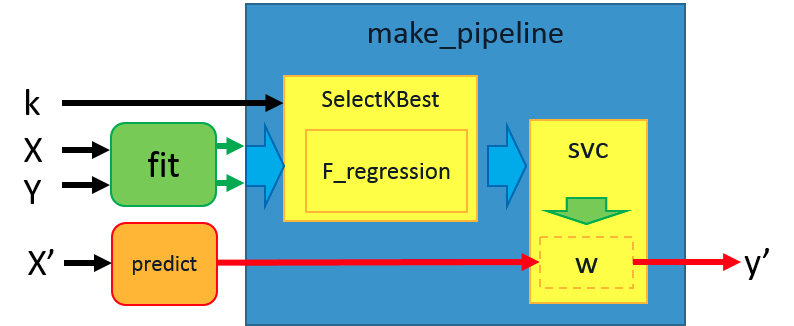
SelectKBest()的第一項參數須給定評分函數,在本範例是設定為f_regression 。第二項參數代表選擇評估分數最高的3個特徵做為訓練的素材。建立完成後,即可用物件內的方法.fit_transform(X,y) 來提取被選出來的特徵。
from sklearn.feature_selection import SelectKBest, f_classiffeature_cols = baseline_data.columns.drop('Installs')# Create the selector, keeping 5 featuresselector = SelectKBest(f_classif, k = 5)# Use the selector to retrieve the best featuresX_new = selector.fit_transform(baseline_data[feature_cols], baseline_data['Installs'])X_new
train, valid, _ = get_data_splits(baseline_data)selector = SelectKBest(f_classif, k = 5)X_new = selector.fit_transform(train[feature_cols], train['Installs'])X_new
# Get back the kept features as a DataFrame with dropped columns as all 0sselected_features = pd.DataFrame(selector.inverse_transform(X_new),index = train.index,columns = feature_cols)selected_features.head()
# Dropped columns have values of all 0s, so var is 0, drop themselected_columns = selected_features.columns[selected_features.var() != 0]# Find the columns that were droppeddropped_columns = selected_features.columns[selected_features.var() == 0]# Get the valid dataset with the selected features.valid[selected_columns].head()
Question
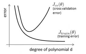
The best value of K
How would you find the “best” value of K?
Solution:
To find the best value of K, you can fit multiple models with increasing values of K, then choose the smallest K with validation score above some threshold or some other criteria.
A good way to do this is loop over values of K and record the validation scores for each iteration.
02 L1 Regularization 正則化 for feature selection
Hint:
First fit the logistic regression model, then pass it to SelectFromModel. That should give you a model with the selected features, you can get the selected features with X_new = model.transform(X).
However, this leaves off the column labels so you’ll need to get them back. The easiest way to do this is to use model.inverse_transform(X_new) to get back the original X array with the dropped columns as all zeros. Then you can create a new DataFrame with the index and columns of X. From there, keep the columns that aren’t all zeros.
Example
def select_features_l1(X, y):logistic = LogisticRegression(C=0.1, penalty="l1", random_state=7).fit(X, y)model = SelectFromModel(logistic, prefit=True)X_new = model.transform(X)# Get back the kept features as a DataFrame with dropped columns as all 0sselected_features = pd.DataFrame(model.inverse_transform(X_new),index=X.index,columns=X.columns)# Dropped columns have values of all 0s, keep other columnscols_to_keep = selected_features.columns[selected_features.var() != 0]return cols_to_keep
03 Feature Selection with Trees
What would you do different to select the features using a trees classifier?
Solution:
You could use something like RandomForestClassifier or ExtraTreesClassifier to find feature importances. SelectFromModel can use the feature importances to find the best features.
04 Top K features with L1 regularization
by setting C you aren’t able to choose a certain number of features to keep. What would you do to keep the top K important features using L1 regularization?
Solution:
To select a certain number of features with L1 regularization, you need to find the regularization parameter that leaves the desired number of features. To do this you can iterate over models with different regularization parameters from low to high and choose the one that leaves K features. Note that for the scikit-learn models C is the inverse of the regularization strength.
Conclusion
首先来说说这几个术语:
特征工程 Feature Engineering:
利用数据领域的相关知识来创建能够使机器学习算法达到最佳性能的特征的过程。
特征构建:
是原始数据中人工的构建新的特征。
特征提取:
自动地构建新的特征,将原始特征转换为一组具有明显物理意义或者统计意义或核的特征。
特征选择:
从特征集合中挑选一组最具统计意义的特征子集,从而达到降维的效果
Feature engineering is a super-set of activities which include feature extraction, feature construction and feature selection. Each of the three are important steps and none should be ignored. We could make a generalization of the importance though, from my experience the relative importance of the steps would be feature construction > feature extraction > feature selection.
特征工程是一个超集,它包括特征提取、特征构建和特征选择这三个子模块。在实践当中,每一个子模块都非常重要,忽略不得。根据答主的经验,他将这三个子模块的重要性进行了一个排名,即:特征构建>特征提取>特征选择。
事实上,真的是这样,如果特征构建做的不好,那么它会直接影响特征提取,进而影响了特征选择,最终影响模型的性能。

若有收获,就点个赞吧
0 人点赞
