下面的范例使用Pytorch的中阶API实现线性回归模型和和DNN二分类模型。
Pytorch的中阶API主要包括各种模型层,损失函数,优化器,数据管道等等。
import osimport datetime#打印时间def printbar():nowtime = datetime.datetime.now().strftime('%Y-%m-%d %H:%M:%S')print("\n"+"=========="*8 + "%s"%nowtime)#mac系统上pytorch和matplotlib在jupyter中同时跑需要更改环境变量os.environ["KMP_DUPLICATE_LIB_OK"]="TRUE"
线性回归模型
准备数据
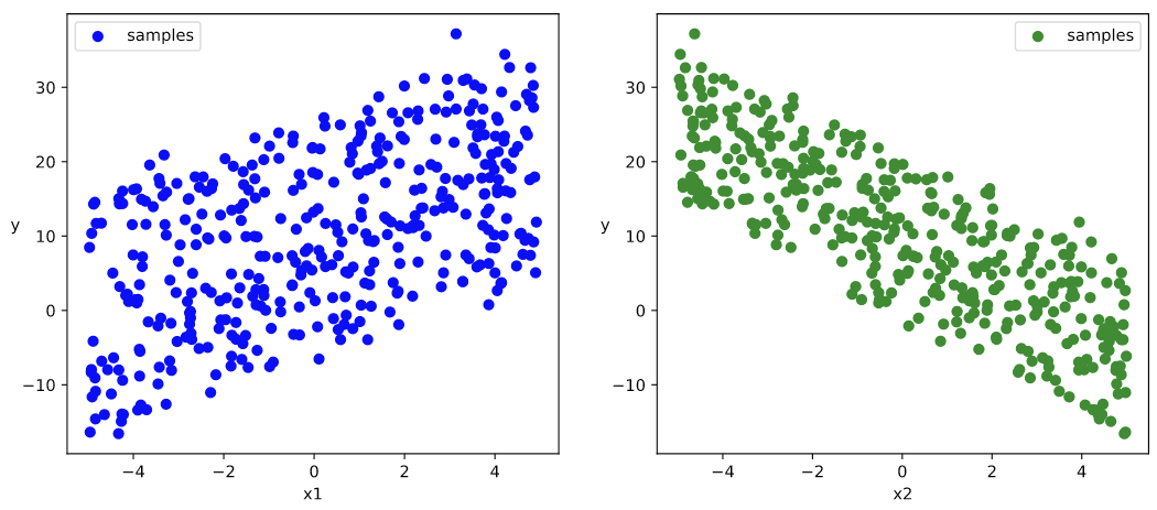
import numpy as npimport pandas as pdfrom matplotlib import pyplot as pltimport torchfrom torch import nnimport torch.nn.functional as Ffrom torch.utils.data import Dataset,DataLoader,TensorDataset#样本数量n = 400# 生成测试用数据集X = 10*torch.rand([n,2])-5.0 #torch.rand是均匀分布w0 = torch.tensor([[2.0],[-3.0]])b0 = torch.tensor([[10.0]])Y = X@w0 + b0 + torch.normal( 0.0,2.0,size = [n,1]) # @表示矩阵乘法,增加正态扰动
# 数据可视化%matplotlib inline%config InlineBackend.figure_format = 'svg'plt.figure(figsize = (12,5))ax1 = plt.subplot(121)ax1.scatter(X[:,0],Y[:,0], c = "b",label = "samples")ax1.legend()plt.xlabel("x1")plt.ylabel("y",rotation = 0)ax2 = plt.subplot(122)ax2.scatter(X[:,1],Y[:,0], c = "g",label = "samples")ax2.legend()plt.xlabel("x2")plt.ylabel("y",rotation = 0)plt.show()# 数据可视化%matplotlib inline%config InlineBackend.figure_format = 'svg'plt.figure(figsize = (12,5))ax1 = plt.subplot(121)ax1.scatter(X[:,0].numpy(),Y[:,0].numpy(), c = "b",label = "samples")ax1.legend()plt.xlabel("x1")plt.ylabel("y",rotation = 0)ax2 = plt.subplot(122)ax2.scatter(X[:,1].numpy(),Y[:,0].numpy(), c = "g",label = "samples")ax2.legend()plt.xlabel("x2")plt.ylabel("y",rotation = 0)plt.show()
#构建输入数据管道ds = TensorDataset(X,Y)ds_train,ds_valid = torch.utils.data.random_split(ds,[int(400*0.7),400-int(400*0.7)])dl_train = DataLoader(ds_train,batch_size = 10,shuffle=True,num_workers=2)dl_valid = DataLoader(ds_valid,batch_size = 10,num_workers=2)
定义模型
model = nn.Linear(2,1) #线性层model.loss_func = nn.MSELoss()model.optimizer = torch.optim.SGD(model.parameters(),lr = 0.01)
训练模型
def train_step(model, features, labels):predictions = model(features)loss = model.loss_func(predictions,labels)loss.backward()model.optimizer.step()model.optimizer.zero_grad()return loss.item()# 测试train_step效果features,labels = next(iter(dl))train_step(model,features,labels)
def train_model(model,epochs):for epoch in range(1,epochs+1):for features, labels in dl:loss = train_step(model,features,labels)if epoch%50==0:printbar()w = model.state_dict()["weight"]b = model.state_dict()["bias"]print("epoch =",epoch,"loss = ",loss)print("w =",w)print("b =",b)train_model(model,epochs = 200)
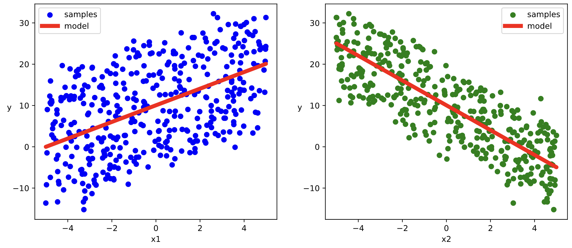
# 结果可视化%matplotlib inline%config InlineBackend.figure_format = 'svg'w,b = model.state_dict()["weight"],model.state_dict()["bias"]plt.figure(figsize = (12,5))ax1 = plt.subplot(121)ax1.scatter(X[:,0],Y[:,0], c = "b",label = "samples")ax1.plot(X[:,0],w[0,0]*X[:,0]+b[0],"-r",linewidth = 5.0,label = "model")ax1.legend()plt.xlabel("x1")plt.ylabel("y",rotation = 0)ax2 = plt.subplot(122)ax2.scatter(X[:,1],Y[:,0], c = "g",label = "samples")ax2.plot(X[:,1],w[0,1]*X[:,1]+b[0],"-r",linewidth = 5.0,label = "model")ax2.legend()plt.xlabel("x2")plt.ylabel("y",rotation = 0)plt.show()
DNN二分类模型
准备数据
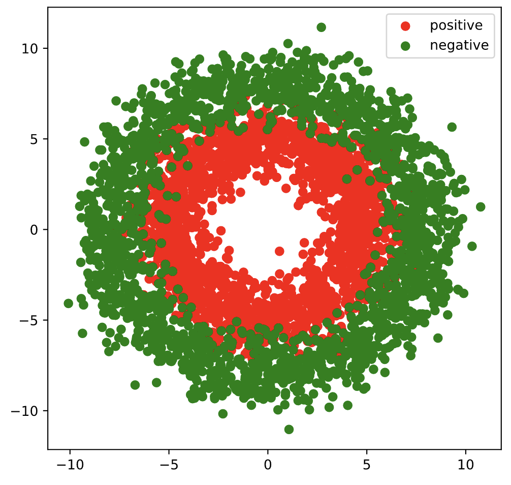
import numpy as npimport pandas as pdfrom matplotlib import pyplot as pltimport torchfrom torch import nn%matplotlib inline%config InlineBackend.figure_format = 'svg'#正负样本数量n_positive,n_negative = 2000,2000#生成正样本, 小圆环分布r_p = 5.0 + torch.normal(0.0,1.0,size = [n_positive,1])theta_p = 2*np.pi*torch.rand([n_positive,1])Xp = torch.cat([r_p*torch.cos(theta_p),r_p*torch.sin(theta_p)],axis = 1)Yp = torch.ones_like(r_p)#生成负样本, 大圆环分布r_n = 8.0 + torch.normal(0.0,1.0,size = [n_negative,1])theta_n = 2*np.pi*torch.rand([n_negative,1])Xn = torch.cat([r_n*torch.cos(theta_n),r_n*torch.sin(theta_n)],axis = 1)Yn = torch.zeros_like(r_n)#汇总样本X = torch.cat([Xp,Xn],axis = 0)Y = torch.cat([Yp,Yn],axis = 0)#可视化plt.figure(figsize = (6,6))plt.scatter(Xp[:,0].numpy(),Xp[:,1].numpy(),c = "r")plt.scatter(Xn[:,0].numpy(),Xn[:,1].numpy(),c = "g")plt.legend(["positive","negative"]);
#构建输入数据管道ds = TensorDataset(X,Y)dl = DataLoader(ds,batch_size = 10,shuffle=True,num_workers=2)
定义模型
class DNNModel(nn.Module):def __init__(self):super(DNNModel, self).__init__()self.fc1 = nn.Linear(2,4)self.fc2 = nn.Linear(4,8)self.fc3 = nn.Linear(8,1)# 正向传播def forward(self,x):x = F.relu(self.fc1(x))x = F.relu(self.fc2(x))y = nn.Sigmoid()(self.fc3(x))return y# 损失函数def loss_func(self,y_pred,y_true):return nn.BCELoss()(y_pred,y_true)# 评估函数(准确率)def metric_func(self,y_pred,y_true):y_pred = torch.where(y_pred>0.5,torch.ones_like(y_pred,dtype = torch.float32),torch.zeros_like(y_pred,dtype = torch.float32))acc = torch.mean(1-torch.abs(y_true-y_pred))return acc# 优化器@propertydef optimizer(self):return torch.optim.Adam(self.parameters(),lr = 0.001)model = DNNModel()
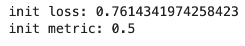
# 测试模型结构(features,labels) = next(iter(dl))predictions = model(features)loss = model.loss_func(predictions,labels)metric = model.metric_func(predictions,labels)print("init loss:",loss.item())print("init metric:",metric.item())# 测试模型结构batch_size = 10(features,labels) = next(data_iter(X,Y,batch_size))predictions = model(features)loss = model.loss_func(labels,predictions)metric = model.metric_func(labels,predictions)print("init loss:", loss.item())print("init metric:", metric.item())
训练模型
def train_step(model, features, labels):# 正向传播求损失predictions = model(features)loss = model.loss_func(predictions,labels)metric = model.metric_func(predictions,labels)# 反向传播求梯度loss.backward()# 更新模型参数model.optimizer.step()model.optimizer.zero_grad()return loss.item(),metric.item()# 测试train_step效果features,labels = next(iter(dl))train_step(model,features,labels)
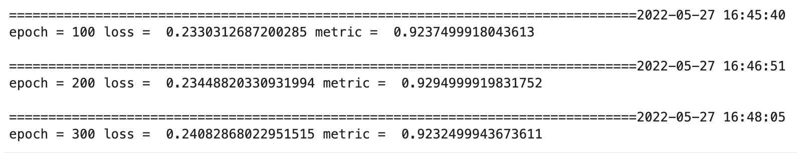
def train_model(model,epochs):for epoch in range(1,epochs+1):loss_list,metric_list = [],[]for features, labels in dl:lossi,metrici = train_step(model,features,labels)loss_list.append(lossi)metric_list.append(metrici)loss = np.mean(loss_list)metric = np.mean(metric_list)if epoch%100==0:printbar()print("epoch =",epoch,"loss = ",loss,"metric = ",metric)train_model(model,epochs = 300)
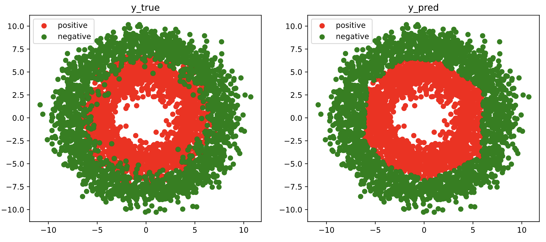
# 结果可视化fig, (ax1,ax2) = plt.subplots(nrows=1,ncols=2,figsize = (12,5))ax1.scatter(Xp[:,0],Xp[:,1], c="r")ax1.scatter(Xn[:,0],Xn[:,1],c = "g")ax1.legend(["positive","negative"]);ax1.set_title("y_true");Xp_pred = X[torch.squeeze(model.forward(X)>=0.5)]Xn_pred = X[torch.squeeze(model.forward(X)<0.5)]ax2.scatter(Xp_pred[:,0],Xp_pred[:,1],c = "r")ax2.scatter(Xn_pred[:,0],Xn_pred[:,1],c = "g")ax2.legend(["positive","negative"]);ax2.set_title("y_pred");

若有收获,就点个赞吧
0 人点赞
