PPT讲义
博客：用PyTorch搭建卷积神经网络
使用PyTorch搭建前馈神经网络对图片进行分类
- 一、数据集
- 二、博客2
导入库
读取展示图片
创建验证集
评估模型
PyTorch的相关库
转换为torch张量
转换为torch张量
训练集形状
博客3

PPT讲义

chap-卷积神经网络.pptx

博客：用PyTorch搭建卷积神经网络

原文地址
在PyTorch中神经网络的构建是通过torch.nn工具
在前馈神经网络已经介绍过autograd，而nn正是基于autograd来定义模型并求取其中的各种梯度

nn.Module定义了网络的每一层
forward(input)则用来计算网络的输出

§ 5. 卷积神经网络 - 图1
来看这样一个用来识别手写体数字的网络，一个典型的训练神经网络的步骤是：

1.定义一个包含一组带学习的参数的神经网络
2.将数据输入到神经网络中并进行前向传播
3.根据损失函数计算输出结果与目标值之间的差距
4.进行梯度反向传播到各个参数
5.更新网络参数，典型的更新方式是：weight = weight - learning_rater * gradient

Define the network

卷积核大小
什么是卷积核？

由这个图我们知道，卷积核指的就是我们要乘得 § 5. 卷积神经网络 - 图5 。

代码

import torch
from torch.autograd import Variable
import torch.nn as nn 
import torch.nn.functional as F
class Net(nn.Module):
    def __init__(self):
        #使用super()方法调用基类的构造器，即nn.Module.__init__(self)
        super(Net,self).__init__()
        '''
        第1个卷积层
        1 input image channel, 6 output channel, 5x5 square convolution kernel
        1个图像通道，因为是灰度图，6个输出频道，应该指的是用6个5x5大小的卷积核(待确定)
        '''
        self.conv1 = nn.Conv2d(1,6,5)
        '''
        第2个卷积层
        6 input channel, 16 output channels, 5x5 square convolution kernel
        这个卷积层应该是连接上一个池化层，所以输入是6个
        然后使用16个5x5大小的卷积层
        '''
        self.conv2 = nn.Conv2d(6,16,5)
        #an affine operation: y = WX+b
        self.fc1 = nn.Linear(16 * 5 * 5,120)
        self.fc2 = nn.Linear(120, 84)
        self.fc3 = nn.Linear(85,10)
    def forward(self,x):
        '''
        x是网络的输入，然后将x前向传播，最后得到输出
        下面两句定义了两个2x2的池化层
        '''
        x = F.max_pool2d(F.relu(self.conv1(x)),(2,2))
        #if the size is square you can only specify a single number
        x = F.max_pool2d(F.relu(self.conv2(x)),2)
        x = x.view(-1,self.num_flat_features(x))
        x = F.relu(self.fc1(x))
        x = F.relu(self.fc2(x))
        x = self.fc3(x)
        return x
    def num_flat_features(self,x):
        size = x.size()[1:] #all dimensions except the batch dimension
        num_features = 1
        for s in size:
            num_features *= s
        return num_features
    net = Net()
    print(net)

以上是定义了一个网络，并且定义了值得前向传播过程，可以进行各种Tensor可以进行的运算，而在梯度反向传播得时候，要用到上章介绍的autograd。

卷积运算

这是卷积核矩阵和输入矩阵中的感受野矩阵之间的内积，也就是两个向量之间的内积，如两个 § 5. 卷积神经网络 - 图6 维向量 § 5. 卷积神经网络 - 图7 和 § 5. 卷积神经网络 - 图8 的内积为
§ 5. 卷积神经网络 - 图9
那么torch.nn.Conv2d()是怎么运算的呢？先来看下它有哪些参数（把这些参数的作用搞清楚，就基本弄清了卷积层的具体工作方式）：

in_channels(int) : Number of channels in the input image.
out_channels(int): Number of channels producted by the convolution.
kernel_size(int or tuple): Size of the convolution. Default: 1.
stride(int or tuple, optional): Zero-padding added to both sides of the input. Default: 0.
dilation(int or tuple, optional): Spacing between kernel elements. Default: 1
groups(int, optional): Number of blocked connections from input channels to output channels. Default: 1
bias(bool, optional): If True, adds a learnable bias to the output. Default: True.

点击这里，PyTorch的详细文档
网络的输入用四元组 § 5. 卷积神经网络 - 图10 来表示，输出表示为 § 5. 卷积神经网络 - 图11 。其中：

和分别表示矩阵的高和宽
表示数据的batch dimension，即批处理的数据一批有多少个
表示输入数据的通道数，按上图中可以理解为输入该层的有几个矩阵
表示输出数据的通道数，可以理解为输出有多少个矩阵

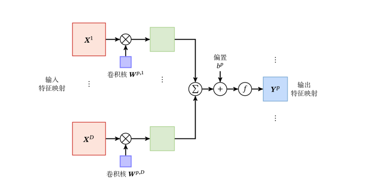
卷积层的输出满足这样的表达式：
§ 5. 卷积神经网络 - 图17
现在只看其中一个数据，即 § 5. 卷积神经网络 - 图18 为一个常数，代表当前数据是batch中的第几个数据，以上面定义的网络的第一个卷积层为例：

§ 5. 卷积神经网络 - 图19
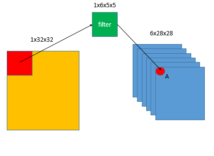
蓝色方框中的红点称为A元素，对这一层上面表达式的各个数值为：

：假设为一批数据中的第1个，即
：输出有6个通道，，对A点
：输入通道，只有1个通道
：是计数器，对应着输入数据的每一个通道，这里只有一个
：偏置参数，维度和一致

卷积核或者说过滤器 § 5. 卷积神经网络 - 图29 是一个 § 5. 卷积神经网络 - 图30 的多维向量， § 5. 卷积神经网络 - 图31 确定了其第一维， § 5. 卷积神经网络 - 图32 确定了其第二维。对于输入向量 § 5. 卷积神经网络 - 图33 ， § 5. 卷积神经网络 - 图34 确定了其第一维。于是求和符号里就是两个向量的内积。当 § 5. 卷积神经网络 - 图35 大于1时，来看第二个卷积层：

§ 5. 卷积神经网络 - 图36
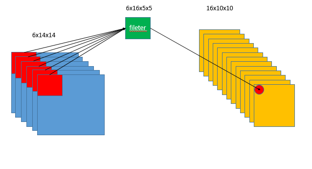
这时 § 5. 卷积神经网络 - 图37 有6个取值，求和符号 § 5. 卷积神经网络 - 图38 中， § 5. 卷积神经网络 - 图39 ，以右侧红点元素为例：当 § 5. 卷积神经网络 - 图40 时是绿色 § 5. 卷积神经网络 - 图41 的向量和左边第一个红色 § 5. 卷积神经网络 - 图42 的向量做内积，然后 § 5. 卷积神经网络 - 图43 是绿色 § 5. 卷积神经网络 - 图44 的向量和第二个红色 § 5. 卷积神经网络 - 图45 的向量做内积，做了6次之后，把这6个内积的结果加和，再加上和第一个输出通道对应的 § 5. 卷积神经网络 - 图46 ，就得到了右侧红点元素的值。
然后左侧红色方框即感受野再按步长移动，输出向量的尺寸是这样的（floor代表向下取整）：
§ 5. 卷积神经网络 - 图47
可以看到上面两个式子涉及到了torch.nn.Conv2d()中的4个参数，kernel_size和stride都好理解，分别是卷积核尺寸和移动步长。

零填充

在网络的早期层中，我们想要尽可能多地保留原始输入内容的信息，这样我们就能提取出那些低层的特征。比如说我们想要应用同样的卷积层，但又想让输出量维持为 32 x 32 x 3 。为做到这点，我们可以对这个层应用大小为 2 的零填充（zero padding）。零填充在输入内容的边界周围补充零。

§ 5. 卷积神经网络 - 图48
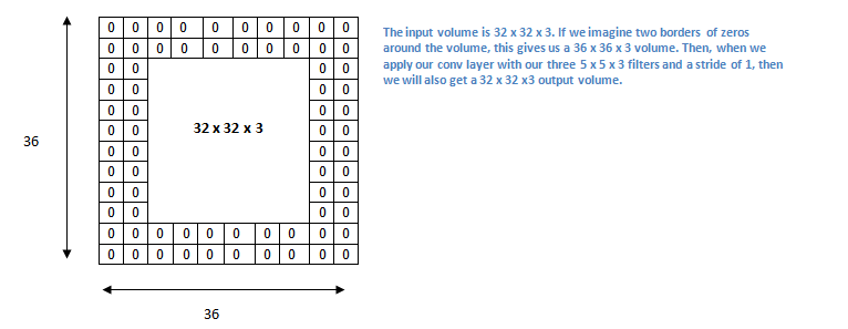
关于padding图片来自这里，这是一个很好的讲解卷积神经网络的文章，还有文字来自对这篇文章翻译的中文版。
dilation：对于这个参数，链接中的最后一个图是关于dilation的。

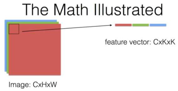
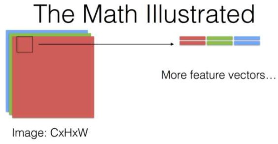
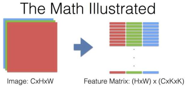
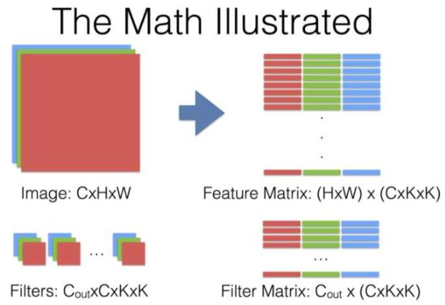
来自这个问题下贾扬清的回答，有几个说明卷积运算过程的图（其中KxK代表卷积核的size，其他符号和上文所用的一致）：

§ 5. 卷积神经网络 - 图50
§ 5. 卷积神经网络 - 图51

§ 5. 卷积神经网络 - 图52
§ 5. 卷积神经网络 - 图53
对于卷积神经网络每一层究竟做了什么，提取出什么特征，这里有个将神经网络可视化的视频

参数个数

对于卷积层来说，参数个数就是 § 5. 卷积神经网络 - 图54 向量和 § 5. 卷积神经网络 - 图55 向量的元素个数和，比如对第二个卷积层来说，就是 § 5. 卷积神经网络 - 图56
可以通过：

net.parameters()

来获得网络的参数。

params = list(net.parameters())
print(len(params))
for i in range(len(params)):
    print(params[i].size())
+++++++++
10
torch.Size([6,1,5,5])
torch.Size([6])
torch.Size([16,6,5,5])
torch.Size([16])
torch.Size([120,400])
torch.Size([120])
torch.Size([84,120])
torch.Size([84])
troch.Size([10,84])
torch.Size([10])
++++++++++

网络的输入与输出

下面来给网络一个输入：

input = Variable(torch.randn(1,1,32,32))
out = net(input)
print(out)
+++++++
Variable containing:
    0.0246 0.0021 -0.0395 -0.0225 -0.0905 -0.0091 -0.0931 -0.0234 -0.1005 0.0795
    [torch.FloatTensor of size 1x10]
+++++++

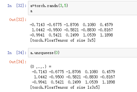
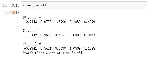
在前面写卷积运算的时候也提到过，实际上网络的输入向量，第一个维度 § 5. 卷积神经网络 - 图57 是批处理数据的个数。在torch.nn方法中必须有这一维的数值，即输入的向量必须是 § 5. 卷积神经网络 - 图58 这样的四维向量。而如果数据没这第一个维度，也就是并不是一批数据，那么可以通过：

torch.Tensor.unsqueeze(0)

在不改变数据所含数值的情况，增加一个维度。
§ 5. 卷积神经网络 - 图59
§ 5. 卷积神经网络 - 图60
§ 5. 卷积神经网络 - 图61

损失函数

如何定义损失函数也很简单的：

output = net(input)
target = Variable(torch.arange(1,11))#a dumy target, for example
criterion = nn.MSELoss() #mean-squared error between the input and target
loss = criterion(output,target)
print(loss)

torch.nn中还有很多损失函数可以使用，点击这里查看

梯度的反向传播

这就要用到autograd.Variable()中的backward()功能。在学习autograd.Variable时也发现，如果Variable.grad已经存储有梯度值，那么当再次写出backward()命令进行梯度回传时，计算出的值将与各个创建变量(graph leaves)的grad已有的值累加。所以对于神经网络，要使用net.zero_grad()清楚掉原有的梯度值。

net.zero_grad() #zeroes the gradient buffers of all parameters
print('conv1.bias.grad before backward')
print(net.conv1.bias.grad)
loss.backward()
print('conv1.bias.grad after backward')
print(net.conv1.bias.grad)

§ 5. 卷积神经网络 - 图62
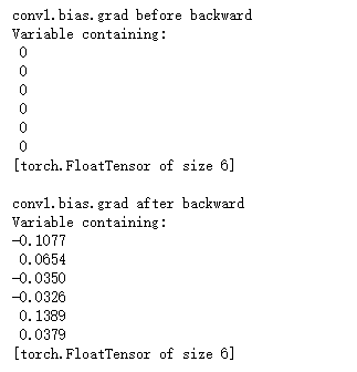
如果原来已有梯度值，然后执行net.zero_grad()，梯度值就变为0，如果原来没有梯度值，那么变量x处的梯度x.grad = None

参数更新

使用torch.optim可以方便的定义参数更新算法：

import torch.optim as optim
#create your optimizer,such as SGD
optimizer = optim.SGD(net.parameters(),lr = 0.01)#lr is learning rate
#in your training loop:
optimizer.zero_grad() #zero the gradient buffers
output = net(input)
loss = criterion(output,target)
loss.backward()
optimizer.step() #Does the update

使用PyTorch搭建前馈神经网络对图片进行分类

原文链接

一、数据集

数据集的来源，该数据集主要是10个种类的衣服，然后90%用作训练集，10%用作测试集。所有图像的大小都是(28*28)的灰度图像。数据集中的两个文件夹，每个都是.csv文件，该文件具有图像的id和相应的标签。
fashion-mnist-master.zip
在PyTorch的手册中，有关于用TensorBoard来训练数据的教程，链接。但是我是在Google Colab中写的代码，所以没有使用这种方式。

二、博客2

这篇博客讲的是使用PyTorch进行的分类。

导入库 ```python
导入库
import pandas as pd import numpy as np

读取展示图片

from skimage.io import imread import matplotlib.pyplot as plt %matplotlib inline

创建验证集

from sklearn.model_selection import train_test_split

评估模型

from sklearn.metrics import accuracy_score from tqdm import tqdm

PyTorch的相关库

import torch from torch.autograd import Variable from torch.nn import Linear, ReLU, CrossEntropyLoss, Sequential, Conv2d, MaxPool2d, Module, Softmax, BatchNorm2d, Dropout from torch.optim import Adam, SGD


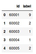
- 加载数据集
现在，让我们加载数据集，包括训练，测试样本：
```python
#加载数据集
train = pd.read_csv('train_LbELTWX/train.csv')
test = pd.read_csv('test_ScVgIM0/test.csv')
sample_submission = pd.read_csv('sample_submission_I5njJSF.csv')
train.head()

§ 5. 卷积神经网络 - 图63

该训练文件包含每个图像的id及其对应的标签
另一方面，测试文件有id，我们必须预测它们对应的标签
样例提交文件将告诉我们预测的格式

我们将一个接一个地读取所有图像，并将它们堆叠成一个数组。我们还将图像的像素值除以255，使图像的像素值在[0,1]范围内。这一步有助于优化模型的性能，让我们来加载图像：

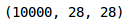
#加载训练图像
train_img = []
for img_name in tqdm(train['id']):
    #定义图像路径
    image_path = 'train_LbELtWX/train/' + str(img_name) + '.png'
    #读取图片
    img = imread(image_path, as_grey=True)
    #归一化像素值
    img /= 255.0
    #转换为浮点数
    img = img.astype('float32')
    #添加到列表
    train_img.append(img)
 #转换为numpy数组
train_x = np.array(train_img)
#定义目标
train_y = train['label'].values
train_x.shape

§ 5. 卷积神经网络 - 图64
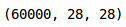
如你所见，我们在训练集中有60，000张大小（28，28）的图像。由于图象是灰度格式的，我们只有一个单一通道，因此形状为(28,28)。现在让我们研究数据和可视化一些图像：

#可视化图片
i = 0
plt.figure(figsize=(10, 10))
plt.subplot(221), plt.imshow(train_x[i], camp='gray')
plt.subplot(222), plt.imshow(train_x[i+25], camp='gray')
plt.subplot(223), plt.imshow(train_x[i+50], camp='gray')
plt.subplot(224), plt.imshow(train_x[i+75], camp='gray')

§ 5. 卷积神经网络 - 图65
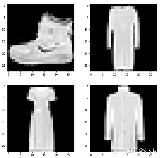
以下是来自数据集的一些示例。接下来，我们把图像分成训练集和验证集。

创建验证集并对图像进行预处理
```
#创建验证集
train_x, val_x, train_y, val_y = train_test_split(train_x,train_y,test_size = 0.1)
(train_x.shape, tain_y.shape), (val_x.shape, val_y.shape)
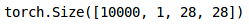
```
我们在验证集中保留了10%的数据，在训练集中保留了10%的数据。接下来将图片和目标转成torch格式： ```python
转换为torch张量
train_x = train_x.reshape(54000, 1, 28, 28) train_x = torch.from_numpy(train_x)

转换为torch张量

train_y = train_y.astype(int); train_y = torch.from_numpy(train_y)

训练集形状

train_x.shape, train_y.shape

![](https://cdn.nlark.com/yuque/0/2020/png/1238812/1597634224803-a1fd3565-9ede-41ab-a9f9-83619ac525b7.png#height=26&id=fXb2i&originHeight=26&originWidth=436&originalType=binary&size=0&status=done&style=none&width=436)<br />同样，我们将转换验证图像：
```python
#转换为torch张量
val_x = val_x.reshape(6000, 1, 28, 28)
val_x = torch.from_numpy(val_x)
#转换为torch张量
val_y = val_y.astype(int);
val_y = torch.from_numpy(val_y)
#验证集形状
val_x.shape, val_y.shape

§ 5. 卷积神经网络 - 图67
我们的数据现在已经准备好了。最后，我们要创建CNN模型。

使用PyTorch实现CNNS

我们将使用一个非常简单的CNN结构，只有两个卷积层来提取图像的特征。然后，我们将使用一个完全连接的Dense层将这些特征分类到各自的类别中，让我们定义一下架构：

class Net(Module):
    def__init__(self):
        super(Net,self).__init__()
        self.cnn_layers = Sequential(
            #define 2D convolution layers
            Conv2d(1, 4, kernel_size=3, stride=1, padding=1),
            BatchNorm2d(4),
            ReLU(inplace=True),
            MaxPool2d(kernel_size=2, stride=2),
            #define another 2d convolution layer
            Conv2d(4, 4, kernel_size_size=3, stride=1, padding=1),
            BatchNorm2d(4),
            ReLU(inplace=True),
            MaxPool2d(kernel_size=2, stride=2),
        )
        self.linear_layers = Sequential(
            Linear(4 * 7 * 7, 10)
        )
        #forward propogation
        def forward(self, x):
            x = self.cnn_layers(x)
            x = x.view(x.size(0), -1)
            x = self.liear_layers(x)
            return x
'''
We call the model defined now, and then define the optimizer and the loss function of the module
'''
#define the module
module = Net()
#define a optimizer
optimizer = Adam(model.parameters(), lr=0.07)
#define the loss function
criterion = CrossEntropyLoss()
#check for the availability of the GPU
if torch.cuda.is_available():
    model = model.cuda()
    criterion = criterion.cuda()
print(model)

§ 5. 卷积神经网络 - 图68
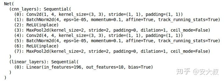
这是模型的架构，我们有两个卷积层和一个线性层。接下来，我们将定义一个函数来训练模型：

def train(epoch):
    model.train()
    tr_loss = 0
    #acquisition the training dataset
    x_train, y_trian = Variable(train_x), Variable(train_y)
    #acqusition the validating dataset
    x_val, y_val = Variabel(val_x), Variable(val_y)
    #transform the variable into GPU format
    if torch.cuda.is_availabel():
        x_train = x_train.cuda()
        y_train = y_train.cuda()
        x_val = x_val.cuda()
        y_val = y_val.cuda()
    #clear the gradient
    optimizer.zero_grad()
    #predict the training and validating dataset
    output_train = model(x_train)
    output_val = model(x_val)
    #calculate the loss of training and validating dataset
    loss_train = criterion(output_train, y_train)
    loss_val = criterion(output_val, y_val)
    train_losses.append(loss_train)
    val_losses.append(loss_val)
    #update the weight
    loss_train.backward()
    optimizer.step()
    tr_loss = lss_train.item()
    if epoch%2 == 0:
        #print the loss of validating dataset
        print('Epoch:',epoch+1,'\t','loss:',loss_val)

最后，我们将对模型进行25个epoch的训练，并存储训练和验证损失：

#define the times of training
n_epochs = 25
#store the loss of training with empty list
train_losses = []
#store the loss of validating with empty list
val_losses = []
#train the module
for epoch in range(n_epochs):
    train(epoch)

§ 5. 卷积神经网络 - 图69
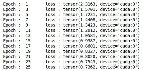
可以看出，随着epoch的增加，验证损失逐渐减小，让我们通过绘图来可视化训练和验证的损失：

#drwa the curve of the loss
plt.plot(train_losses, label='Training loss')
plt.plot(val_losses, label='Validation loss')
plt.legend()
plt.show()

§ 5. 卷积神经网络 - 图70
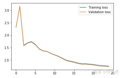
我们可以清楚地看到，训练和验证损失是同步的，这是一个好迹象，因为模型在验证集上进行了很好的泛化。让我们在训练和验证集上检查模型的准确性：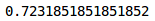
§ 5. 卷积神经网络 - 图71

#prediction of the training dataset
with torch.no_grad():
    output = model(train_x.cuda())
softmax = torch.exp(output).cpu()
prob = list(softmax.numpy())
predictions = np.argmax(prob, axis=1)
#the accuracy of training dataset
accuracy_score(train_y,predictions)

§ 5. 卷积神经网络 - 图72
训练集的准确率约为72%，相当不错。让我们来检查验证集的准确性：

# prediction of validation dataset
with torch.no_grad():
    output = model(val_x.cuda())
softmax = torch.exp(output).cpu()
prob = list(softmax.numpy())
predictions = np.argmax(prob, axis=1)
#the accuracy of validation dataset
accuracy_score(val_y, predictions)

§ 5. 卷积神经网络 - 图73
正如我们看到的损失，准确度也是同步的，我们在验证集得到了72%的准确度。

为验证集生成预测

最后为测试机生成预测。我们将加载测试集中的所有图像，执行与训练集相同的预处理步骤，最后生成预测。所以，让我们开始加载测试图像：

#load the training images
test_img = []
for img_name in tqdm(test['id']):
    #define the path of images
    image_path = 'test_ScVgIM0/test/' + str(img_name) + '.png'
    #read the picture
    img = imread(image_path, as_gray=True)
    #normalize the pixel
    img /= 255.0
    #transform  the dtype of image into float
    img = img.astype('float32')
    #add the image to list
    test_img.append(img)
#transform the "test_img" into numpy arrsy
test_x = np.array(test_img)
test_x.shape

§ 5. 卷积神经网络 - 图74
现在，我们将对这些图像进行预处理步骤，类似于我们之前对训练图像所做的：

#transform the "test_x" into torch format
test_x = test_x.reshape(10000, 1, 28, 28)
test_x = torch.from_numpy(test_x)
test_x.shape

§ 5. 卷积神经网络 - 图75
最后，我们将生成对测试集的预测：

#generate the prediction of training dataset
with torch.no_grad():
    output = model(test_x.cuda())
softmax = torch.exp(output).cpu()
prob = list(softmax.numpy())
predicitons = np.argmax(prob, axis=1)

用预测替换样本提交文件中的标签，最后保存文件并提交到排行榜

#replace the label of sample submission file with prediction 
sample_submission['label'] = predictions
sample_submission.head()

§ 5. 卷积神经网络 - 图76

#save the file
sample_submission.to_csv('submission.csv',index=False)

你将在当前目录中看到一个名为submission.csv的文件。你只需要把它上传到问题页面的解决方案检查器上，它就会生成分数,点击链接。我们的CNN模型在测试集上给出了大约71%的准确率，这与我们在上一篇文章中使用简单的神经网络得到的65%的准确率相比是一个很大的进步。

结尾

在这篇文章中，我们研究了CNNs是如何从图像中提取特征的。他们帮助我们将之前的神经网络模型的准确率从65%提高到71%，这是一个重大的进步。你可以尝试使用CNN模型的超参数，并尝试进一步提高准确性。要调优的超参数可以是卷积层的数量、每个卷积层的滤波器数量、epoch的数量、全连接层的数量、每个全连接层的隐藏单元的数量等。

博客3

原文链接

§ 5. 卷积神经网络

PPT讲义

博客：用PyTorch搭建卷积神经网络

Define the network

卷积核大小

代码

卷积运算

零填充

参数个数

网络的输入与输出

损失函数

梯度的反向传播

参数更新

使用PyTorch搭建前馈神经网络对图片进行分类

一、数据集

二、博客2

导入库

读取展示图片

创建验证集

评估模型

PyTorch的相关库

转换为torch张量

转换为torch张量

训练集形状

博客3