空间变压器网络教程
原文: https://pytorch.org/tutorials/intermediate/spatial_transformer_tutorial.html
注意
单击此处的下载完整的示例代码
作者: Ghassen HAMROUNI
在本教程中,您将学习如何使用称为空间变换器网络的视觉注意力机制来扩充网络。 您可以在 DeepMind 论文中详细了解空间变压器网络。
空间变换器网络是对任何空间变换的可区别关注的概括。 空间变换器网络(简称 STN)允许神经网络学习如何对输入图像执行空间变换,以增强模型的几何不变性。 例如,它可以裁剪感兴趣的区域,缩放并校正图像的方向。 这可能是一个有用的机制,因为 CNN 不会对旋转和缩放以及更一般的仿射变换保持不变。
关于 STN 的最好的事情之一就是能够将它简单地插入到任何现有的 CNN 中。
# License: BSD# Author: Ghassen Hamrounifrom __future__ import print_functionimport torchimport torch.nn as nnimport torch.nn.functional as Fimport torch.optim as optimimport torchvisionfrom torchvision import datasets, transformsimport matplotlib.pyplot as pltimport numpy as npplt.ion() # interactive mode
加载数据
在本文中,我们将尝试使用经典的 MNIST 数据集。 使用标准卷积网络和空间变换器网络。
device = torch.device("cuda" if torch.cuda.is_available() else "cpu")# Training datasettrain_loader = torch.utils.data.DataLoader(datasets.MNIST(root='.', train=True, download=True,transform=transforms.Compose([transforms.ToTensor(),transforms.Normalize((0.1307,), (0.3081,))])), batch_size=64, shuffle=True, num_workers=4)# Test datasettest_loader = torch.utils.data.DataLoader(datasets.MNIST(root='.', train=False, transform=transforms.Compose([transforms.ToTensor(),transforms.Normalize((0.1307,), (0.3081,))])), batch_size=64, shuffle=True, num_workers=4)
出:
Downloading http://yann.lecun.com/exdb/mnist/train-images-idx3-ubyte.gz to ./MNIST/raw/train-images-idx3-ubyte.gzExtracting ./MNIST/raw/train-images-idx3-ubyte.gz to ./MNIST/rawDownloading http://yann.lecun.com/exdb/mnist/train-labels-idx1-ubyte.gz to ./MNIST/raw/train-labels-idx1-ubyte.gzExtracting ./MNIST/raw/train-labels-idx1-ubyte.gz to ./MNIST/rawDownloading http://yann.lecun.com/exdb/mnist/t10k-images-idx3-ubyte.gz to ./MNIST/raw/t10k-images-idx3-ubyte.gzExtracting ./MNIST/raw/t10k-images-idx3-ubyte.gz to ./MNIST/rawDownloading http://yann.lecun.com/exdb/mnist/t10k-labels-idx1-ubyte.gz to ./MNIST/raw/t10k-labels-idx1-ubyte.gzExtracting ./MNIST/raw/t10k-labels-idx1-ubyte.gz to ./MNIST/rawProcessing...Done!
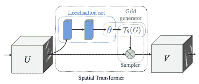
描述空间变压器网络
空间变压器网络可归结为三个主要组成部分:
- 本地化网络是常规的 CNN,可以对转换参数进行回归。 永远不会从此数据集中显式学习变换,而是网络会自动学习增强全局精度的空间变换。
- 网格生成器在输入图像中生成与来自输出图像的每个像素相对应的坐标网格。
- 采样器使用转换的参数,并将其应用于输入图像。
Note
我们需要包含 affine_grid 和 grid_sample 模块的最新版本的 PyTorch。
class Net(nn.Module):def __init__(self):super(Net, self).__init__()self.conv1 = nn.Conv2d(1, 10, kernel_size=5)self.conv2 = nn.Conv2d(10, 20, kernel_size=5)self.conv2_drop = nn.Dropout2d()self.fc1 = nn.Linear(320, 50)self.fc2 = nn.Linear(50, 10)# Spatial transformer localization-networkself.localization = nn.Sequential(nn.Conv2d(1, 8, kernel_size=7),nn.MaxPool2d(2, stride=2),nn.ReLU(True),nn.Conv2d(8, 10, kernel_size=5),nn.MaxPool2d(2, stride=2),nn.ReLU(True))# Regressor for the 3 * 2 affine matrixself.fc_loc = nn.Sequential(nn.Linear(10 * 3 * 3, 32),nn.ReLU(True),nn.Linear(32, 3 * 2))# Initialize the weights/bias with identity transformationself.fc_loc[2].weight.data.zero_()self.fc_loc[2].bias.data.copy_(torch.tensor([1, 0, 0, 0, 1, 0], dtype=torch.float))# Spatial transformer network forward functiondef stn(self, x):xs = self.localization(x)xs = xs.view(-1, 10 * 3 * 3)theta = self.fc_loc(xs)theta = theta.view(-1, 2, 3)grid = F.affine_grid(theta, x.size())x = F.grid_sample(x, grid)return xdef forward(self, x):# transform the inputx = self.stn(x)# Perform the usual forward passx = F.relu(F.max_pool2d(self.conv1(x), 2))x = F.relu(F.max_pool2d(self.conv2_drop(self.conv2(x)), 2))x = x.view(-1, 320)x = F.relu(self.fc1(x))x = F.dropout(x, training=self.training)x = self.fc2(x)return F.log_softmax(x, dim=1)model = Net().to(device)
训练模型
现在,让我们使用 SGD 算法训练模型。 网络正在以监督方式学习分类任务。 同时,该模型以端到端的方式自动学习 STN。
optimizer = optim.SGD(model.parameters(), lr=0.01)def train(epoch):model.train()for batch_idx, (data, target) in enumerate(train_loader):data, target = data.to(device), target.to(device)optimizer.zero_grad()output = model(data)loss = F.nll_loss(output, target)loss.backward()optimizer.step()if batch_idx % 500 == 0:print('Train Epoch: {} [{}/{} ({:.0f}%)]\tLoss: {:.6f}'.format(epoch, batch_idx * len(data), len(train_loader.dataset),100\. * batch_idx / len(train_loader), loss.item()))## A simple test procedure to measure STN the performances on MNIST.#def test():with torch.no_grad():model.eval()test_loss = 0correct = 0for data, target in test_loader:data, target = data.to(device), target.to(device)output = model(data)# sum up batch losstest_loss += F.nll_loss(output, target, size_average=False).item()# get the index of the max log-probabilitypred = output.max(1, keepdim=True)[1]correct += pred.eq(target.view_as(pred)).sum().item()test_loss /= len(test_loader.dataset)print('\nTest set: Average loss: {:.4f}, Accuracy: {}/{} ({:.0f}%)\n'.format(test_loss, correct, len(test_loader.dataset),100\. * correct / len(test_loader.dataset)))
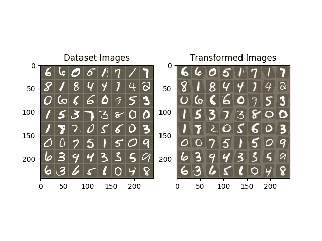
可视化 STN 结果
现在,我们将检查学习到的视觉注意力机制的结果。
我们定义了一个小的辅助函数,以便在训练时可视化转换。
def convert_image_np(inp):"""Convert a Tensor to numpy image."""inp = inp.numpy().transpose((1, 2, 0))mean = np.array([0.485, 0.456, 0.406])std = np.array([0.229, 0.224, 0.225])inp = std * inp + meaninp = np.clip(inp, 0, 1)return inp# We want to visualize the output of the spatial transformers layer# after the training, we visualize a batch of input images and# the corresponding transformed batch using STN.def visualize_stn():with torch.no_grad():# Get a batch of training datadata = next(iter(test_loader))[0].to(device)input_tensor = data.cpu()transformed_input_tensor = model.stn(data).cpu()in_grid = convert_image_np(torchvision.utils.make_grid(input_tensor))out_grid = convert_image_np(torchvision.utils.make_grid(transformed_input_tensor))# Plot the results side-by-sidef, axarr = plt.subplots(1, 2)axarr[0].imshow(in_grid)axarr[0].set_title('Dataset Images')axarr[1].imshow(out_grid)axarr[1].set_title('Transformed Images')for epoch in range(1, 20 + 1):train(epoch)test()# Visualize the STN transformation on some input batchvisualize_stn()plt.ioff()plt.show()
Out:
Train Epoch: 1 [0/60000 (0%)] Loss: 2.312544Train Epoch: 1 [32000/60000 (53%)] Loss: 0.865688Test set: Average loss: 0.2105, Accuracy: 9426/10000 (94%)Train Epoch: 2 [0/60000 (0%)] Loss: 0.528199Train Epoch: 2 [32000/60000 (53%)] Loss: 0.273284Test set: Average loss: 0.1150, Accuracy: 9661/10000 (97%)Train Epoch: 3 [0/60000 (0%)] Loss: 0.312562Train Epoch: 3 [32000/60000 (53%)] Loss: 0.496166Test set: Average loss: 0.1130, Accuracy: 9661/10000 (97%)Train Epoch: 4 [0/60000 (0%)] Loss: 0.346181Train Epoch: 4 [32000/60000 (53%)] Loss: 0.206084Test set: Average loss: 0.0875, Accuracy: 9730/10000 (97%)Train Epoch: 5 [0/60000 (0%)] Loss: 0.351175Train Epoch: 5 [32000/60000 (53%)] Loss: 0.388225Test set: Average loss: 0.0659, Accuracy: 9802/10000 (98%)Train Epoch: 6 [0/60000 (0%)] Loss: 0.122667Train Epoch: 6 [32000/60000 (53%)] Loss: 0.258372Test set: Average loss: 0.0791, Accuracy: 9759/10000 (98%)Train Epoch: 7 [0/60000 (0%)] Loss: 0.190197Train Epoch: 7 [32000/60000 (53%)] Loss: 0.154468Test set: Average loss: 0.0647, Accuracy: 9791/10000 (98%)Train Epoch: 8 [0/60000 (0%)] Loss: 0.121149Train Epoch: 8 [32000/60000 (53%)] Loss: 0.288490Test set: Average loss: 0.0583, Accuracy: 9821/10000 (98%)Train Epoch: 9 [0/60000 (0%)] Loss: 0.244609Train Epoch: 9 [32000/60000 (53%)] Loss: 0.023396Test set: Average loss: 0.0685, Accuracy: 9778/10000 (98%)Train Epoch: 10 [0/60000 (0%)] Loss: 0.256878Train Epoch: 10 [32000/60000 (53%)] Loss: 0.091626Test set: Average loss: 0.0684, Accuracy: 9783/10000 (98%)Train Epoch: 11 [0/60000 (0%)] Loss: 0.181910Train Epoch: 11 [32000/60000 (53%)] Loss: 0.113193Test set: Average loss: 0.0492, Accuracy: 9856/10000 (99%)Train Epoch: 12 [0/60000 (0%)] Loss: 0.081072Train Epoch: 12 [32000/60000 (53%)] Loss: 0.082513Test set: Average loss: 0.0670, Accuracy: 9800/10000 (98%)Train Epoch: 13 [0/60000 (0%)] Loss: 0.180748Train Epoch: 13 [32000/60000 (53%)] Loss: 0.194512Test set: Average loss: 0.0439, Accuracy: 9874/10000 (99%)Train Epoch: 14 [0/60000 (0%)] Loss: 0.099560Train Epoch: 14 [32000/60000 (53%)] Loss: 0.084377Test set: Average loss: 0.0416, Accuracy: 9880/10000 (99%)Train Epoch: 15 [0/60000 (0%)] Loss: 0.070021Train Epoch: 15 [32000/60000 (53%)] Loss: 0.241336Test set: Average loss: 0.0588, Accuracy: 9820/10000 (98%)Train Epoch: 16 [0/60000 (0%)] Loss: 0.060536Train Epoch: 16 [32000/60000 (53%)] Loss: 0.053016Test set: Average loss: 0.0405, Accuracy: 9877/10000 (99%)Train Epoch: 17 [0/60000 (0%)] Loss: 0.207369Train Epoch: 17 [32000/60000 (53%)] Loss: 0.069607Test set: Average loss: 0.1006, Accuracy: 9685/10000 (97%)Train Epoch: 18 [0/60000 (0%)] Loss: 0.127503Train Epoch: 18 [32000/60000 (53%)] Loss: 0.070724Test set: Average loss: 0.0659, Accuracy: 9814/10000 (98%)Train Epoch: 19 [0/60000 (0%)] Loss: 0.176861Train Epoch: 19 [32000/60000 (53%)] Loss: 0.116980Test set: Average loss: 0.0413, Accuracy: 9871/10000 (99%)Train Epoch: 20 [0/60000 (0%)] Loss: 0.146933Train Epoch: 20 [32000/60000 (53%)] Loss: 0.245741Test set: Average loss: 0.0346, Accuracy: 9892/10000 (99%)
脚本的总运行时间:(2 分钟 3.339 秒)
Download Python source code: spatial_transformer_tutorial.py Download Jupyter notebook: spatial_transformer_tutorial.ipynb
由狮身人面像画廊生成的画廊

若有收获,就点个赞吧
0 人点赞
