torch.nn

torch.nn

译者：@小王子、@那伊抹微笑、@Yang Shun、@Zhu Yansen、@woaichipinngguo、@buldajs、@吉思雨、@王云峰、@李雨龙、@Yucong Zhu、@林嘉应、@QianFanCe、@dabney777、@Alex、@SiKai Yao、@小乔 @laihongchang @噼里啪啦嘣 @BarrettLi、@KrokYin、@MUSK1881

校对者：@clown9804、@飞龙

Parameters (参数)

class torch.nn.Parameter

Variable 的一种, 常被用于 module parameter(模块参数）.

Parameters 是 Variable](autograd.html#torch.autograd.Variable “torch.autograd.Variable”) 的子类, 当它和 [Module 一起使用的时候会有一些特殊的属性 - 当它们被赋值给 Module 属性时, 它会自动的被加到 Module 的参数列表中, 并且会出现在 parameters() iterator 迭代器方法中. 将 Varibale 赋值给 Module 属性则不会有这样的影响. 这样做的原因是: 我们有时候会需要缓存一些临时的 state(状态）, 例如: 模型 RNN 中的最后一个隐藏状态. 如果没有 Parameter 这个类的话, 那么这些临时表也会注册为模型变量.

Variable 与 Parameter 的另一个不同之处在于, Parameter 不能被 volatile (即: 无法设置 volatile=True) 而且默认 requires_grad=True. Variable 默认 requires_grad=False.

参数：

data (Tensor) – parameter tensor.
requires_grad (bool, 可选) – 如果参数需要梯度. 更多细节请参阅反向排除 subgraphs (子图).

Containers (容器)

Module

class torch.nn.Module

所有神经网络的基类.

你的模型应该也是该类的子类.

Modules 也可以包含其它 Modules, 允许使用树结构嵌入它们. 你可以将子模块赋值给模型属性

import torch.nn as nn
import torch.nn.functional as F
class Model(nn.Module):
    def __init__(self):
        super(Model, self).__init__()
        self.conv1 = nn.Conv2d(1, 20, 5)
        self.conv2 = nn.Conv2d(20, 20, 5)
    def forward(self, x):
       x = F.relu(self.conv1(x))
       return F.relu(self.conv2(x))

以这种方式分配的子模块将被注册, 并且在调用 .cuda() 等等方法时也将转换它们的参数.

add_module(name, module)

添加一个 child module(子模块）到当前的 module(模块）中.

被添加的 module 还可以通过指定的 name 属性来获取它.

参数：

name (string) – 子模块的名称. 可以使用指定的 name 从该模块访问子模块
parameter (Module) – 被添加到模块的子模块.

apply(fn)

将 fn 函数递归的应用到每一个子模块 (由 .children() 方法所返回的) 以及 self. 典型的用于包括初始化模型的参数 (也可参阅 torch-nn-init).

参数：fn (Module -> None) – 要被应用到每一个子模块上的函数

返回值：self

返回类型：Module

示例：

>>> def init_weights(m):
>>>     print(m)
>>>     if type(m) == nn.Linear:
>>>         m.weight.data.fill_(1.0)
>>>         print(m.weight)
>>>
>>> net = nn.Sequential(nn.Linear(2, 2), nn.Linear(2, 2))
>>> net.apply(init_weights)
Linear (2 -> 2)
Parameter containing:
 1  1
 1  1
[torch.FloatTensor of size 2x2]
Linear (2 -> 2)
Parameter containing:
 1  1
 1  1
[torch.FloatTensor of size 2x2]
Sequential (
 (0): Linear (2 -> 2)
 (1): Linear (2 -> 2)
)

children()

返回一个最近子模块的 iterator(迭代器）.

Yields: Module – 一个子模块

cpu()

将所有的模型参数和缓冲区移动到 CPU.

返回值：self

返回类型：Module

cuda(device=None)

将所有的模型参数和缓冲区移动到 GPU.

这将会关联一些参数并且缓存不同的对象. 所以在构建优化器之前应该调用它, 如果模块在优化的情况下会生存在 GPU 上.

参数：device (int, 可选) – 如果指定, 所有参数将被复制到指定的设备上

返回值：self

返回类型：Module

double()

将所有的 parameters 和 buffers 的数据类型转换成 double.

返回值：self

返回类型：Module

eval()

将模块设置为评估模式.

这种方式只对 Dropout 或 BatchNorm 等模块有效.

float()

将所有的 parameters 和 buffers 的数据类型转换成float.

返回值：self

返回类型：Module

forward(*input)

定义每次调用时执行的计算.

应该被所有的子类重写.

注解：

尽管需要在此函数中定义正向传递的方式, 但是应该事后尽量调用 Module 实例, 因为前者负责运行已注册的钩子, 而后者静默的忽略它们.

half()

将所有的 parameters 和 buffers 的数据类型转换成 half.

返回值：self

返回类型：Module

load_state_dict(state_dict, strict=True)

将 state_dict 中的 parameters 和 buffers 复制到此模块和它的子后代中. 如果 strict 为 True, 则 state_dict 的 key 必须和模块的 state_dict() 函数返回的 key 一致.

参数：

state_dict (dict) – 一个包含 parameters 和 persistent buffers(持久化缓存的）字典.
strict (bool) – 严格的强制 state_dict 属性中的 key 与该模块的函数 state_dict() 返回的 keys 相匹配.

modules()

返回一个覆盖神经网络中所有模块的 iterator(迭代器）.

Yields: Module – 网络中的一个模块

注解：

重复的模块只返回一次. 在下面的例子中, 1 只会被返回一次. example, l will be returned only once.

>>> l = nn.Linear(2, 2)
>>> net = nn.Sequential(l, l)
>>> for idx, m in enumerate(net.modules()):
>>>     print(idx, '->', m)
0 -> Sequential (
 (0): Linear (2 -> 2)
 (1): Linear (2 -> 2)
)
1 -> Linear (2 -> 2)

named_children()

返回一个 iterator(迭代器）, 而不是最接近的子模块, 产生模块的 name 以及模块本身.

Yields: (string, Module) – 包含名称和子模块的 Tuple(元组）

示例：

>>> for name, module in model.named_children():
>>>     if name in ['conv4', 'conv5']:
>>>         print(module)

named_modules(memo=None, prefix='')

返回一个神经网络中所有模块的 iterator(迭代器）, 产生模块的 name 以及模块本身.

Yields: (string, Module) – 名字和模块的 Tuple(元组）

注解：

重复的模块只返回一次. 在下面的例子中, 1 只会被返回一次.

>>> l = nn.Linear(2, 2)
>>> net = nn.Sequential(l, l)
>>> for idx, m in enumerate(net.named_modules()):
>>>     print(idx, '->', m)
0 -> ('', Sequential (
 (0): Linear (2 -> 2)
 (1): Linear (2 -> 2)
))
1 -> ('0', Linear (2 -> 2))

named_parameters(memo=None, prefix='')

返回模块参数的迭代器, 产生参数的名称以及参数本身

Yields: (string, Parameter) – Tuple 包含名称很参数的 Tuple(元组）

示例：

>>> for name, param in self.named_parameters():
>>>    if name in ['bias']:
>>>        print(param.size())

parameters()

返回一个模块参数的迭代器.

这通常传递给优化器.

Yields: Parameter – 模型参数

示例：

>>> for param in model.parameters():
>>>     print(type(param.data), param.size())
<class 'torch.FloatTensor'> (20L,)
<class 'torch.FloatTensor'> (20L, 1L, 5L, 5L)

register_backward_hook(hook)

在模块上注册一个 backward hook(反向钩子）.

每次计算关于模块输入的梯度时, 都会调用该钩子. 钩子应该有以下结构:

hook(module, grad_input, grad_output) -> Tensor or None

如果 module 有多个输入或输出的话, 那么 grad_input 和 grad_output 将会是个 tuple. hook 不应该修改它的参数, 但是它可以选择性地返回一个新的关于输入的梯度, 这个返回的梯度在后续的计算中会替代 grad_input.

返回值：通过调用 handle.remove() 方法可以删除添加钩子的句柄 handle.remove()

返回类型：torch.utils.hooks.RemovableHandle

register_buffer(name, tensor)

给模块添加一个持久化的 buffer.

持久化的 buffer 通常被用在这么一种情况: 我们需要保存一个状态, 但是这个状态不能看作成为模型参数. 例如: BatchNorm 的 running_mean 不是一个 parameter, 但是它也是需要保存的状态之一.

Buffers 可以使用指定的 name 作为属性访问.

参数：

name (string) – buffer 的名称. 可以使用指定的 name 从该模块访问 buffer
tensor (Tensor) – 被注册的 buffer.

示例：

>>> self.register_buffer('running_mean', torch.zeros(num_features))

register_forward_hook(hook)

在模块上注册一个 forward hook(前向钩子）.

每一次 forward() 函数计算出一个输出后, 该钩子将会被调用. 它应该具有以下结构

hook(module, input, output) -> None

该钩子应该不会修改输入或输出.

返回值：通过调用 handle.remove() 方法可以删除添加钩子的句柄

返回类型：torch.utils.hooks.RemovableHandle

register_forward_pre_hook(hook)

在模块上注册一个预前向钩子.

每一次在调用 forward() 函数前都会调用该钩子. 它应该有以下结构:

hook(module, input) -> None

该钩子不应该修改输入.

返回值：通过调用 handle.remove() 方法可以删除添加钩子的句柄 handle.remove()

返回类型：torch.utils.hooks.RemovableHandle

register_parameter(name, param)

添加一个参数到模块中.

可以使用指定的 name 属性来访问参数.

参数：

name (string) – 参数名. 可以使用指定的 name 来从该模块中访问参数
parameter (Parameter) – 要被添加到模块的参数.

state_dict(destination=None, prefix='', keep_vars=False)

返回一个字典, 它包含整个模块的状态.

包括参数和持久化的缓冲区 (例如. 运行中的平均值). Keys 是与之对应的参数和缓冲区的 name.

当 keep_vars 为 True 时, 它为每一个参数(而不是一个张量）返回一个 Variable.

参数：

destination (dict, 可选) – 如果不是 None, 该返回的字典应该被存储到 destination 中. Default: None
prefix (string, 可选) – 向结果字典中的每个参数和缓冲区的 key(名称）添加一个前缀. Default: ‘’
keep_vars (bool, 可选) – 如果为 True, 为每一个参数返回一个 Variable. 如果为 False, 为每一个参数返回一个 Tensor. Default: False

返回值：包含模块整体状态的字典

返回类型：dict

示例：

>>> module.state_dict().keys()
['bias', 'weight']

train(mode=True)

设置模块为训练模式.

这只对诸如 Dropout 或 BatchNorm 等模块时才会有影响.

返回值：self

返回类型：Module

type(dst_type)

转换所有参数和缓冲区为 dst_type.

参数：dst_type (type 或 string) – 理想的类型

返回值：self

返回类型：Module

zero_grad()

将所有模型参数的梯度设置为零.

Sequential

class torch.nn.Sequential(*args)

一个顺序的容器. 模块将按照它们在构造函数中传递的顺序添加到它. 或者, 也可以传入模块的有序字典.

为了更容易理解, 列举小例来说明

# 使用 Sequential 的例子
model = nn.Sequential(
          nn.Conv2d(1,20,5),
          nn.ReLU(),
          nn.Conv2d(20,64,5),
          nn.ReLU()
        )
# 与 OrderedDict 一起使用 Sequential 的例子
model = nn.Sequential(OrderedDict([
          ('conv1', nn.Conv2d(1,20,5)),
          ('relu1', nn.ReLU()),
          ('conv2', nn.Conv2d(20,64,5)),
          ('relu2', nn.ReLU())
        ]))

ModuleList

class torch.nn.ModuleList(modules=None)

将子模块放入一个 list 中.

ModuleList 可以像普通的 Python list 一样被索引, 但是它包含的模块已经被正确的注册了, 并且所有的 Module 方法都是可见的.

参数：modules (list, 可选) – 要添加的模块列表

示例：

class MyModule(nn.Module):
    def __init__(self):
        super(MyModule, self).__init__()
        self.linears = nn.ModuleList([nn.Linear(10, 10) for i in range(10)])
    def forward(self, x):
        # ModuleList can act as an iterable, or be indexed using ints
        for i, l in enumerate(self.linears):
            x = self.linears[i // 2](x) + l(x)
        return x

append(module)

添加一个指定的模块到 list 尾部.

参数：module (nn.Module) – 要被添加的模块

extend(modules)

在最后添加 Python list 中的模块.

参数：modules (list) – 要被添加的模块列表

ParameterList

class torch.nn.ParameterList(parameters=None)

保存 list 中的 parameter.

ParameterList 可以像普通的 Python list 那样被索引, 但是它所包含的参数被正确的注册了, 并且所有的 Module 方法都可见的.

参数：modules (list, 可选) – 要被添加的 Parameter 列表

示例：

class MyModule(nn.Module):
    def __init__(self):
        super(MyModule, self).__init__()
        self.params = nn.ParameterList([nn.Parameter(torch.randn(10, 10)) for i in range(10)])
    def forward(self, x):
        # ModuleList 可以充当 iterable(迭代器）, 或者可以使用整数进行索引
        for i, p in enumerate(self.params):
            x = self.params[i // 2].mm(x) + p.mm(x)
        return x

append(parameter)

添加一个指定的参数到 list 尾部.

参数：parameter (nn.Parameter) – parameter to append

extend(parameters)

在最后添加 Python list 中的参数.

参数：parameters (list) – list of parameters to append

Convolution Layers (卷积层)

Conv1d

class torch.nn.Conv1d(in_channels, out_channels, kernel_size, stride=1, padding=0, dilation=1, groups=1, bias=True)

一维卷积层输入矩阵的维度为 $(N, C_{in}, L)$ , 输出矩阵维度为 $(N, C_{out}, L_{out})$ . 其中N为输入数量, C为每个输入样本的通道数量, L为样本中一个通道下的数据的长度. 算法如下:

$\begin{array}{ll} out(N_i, C_{out_j}) = bias(C_{out_j}) + \sum_{k=0}^{C_{in}-1} weight(C_{out_j}, k) \star input(N_i, k) \end{array}$

$\star$ 是互相关运算符, 上式带 $\star$ 项为卷积项.

stride 计算相关系数的步长, 可以为 tuple .padding 处理边界时在两侧补0数量dilation 采样间隔数量. 大于1时为非致密采样, 如对(a,b,c,d,e)采样时, 若池化规模为2,

dilation 为1时, 使用 (a,b);(b,c)… 进行池化, dilation 为1时, 使用 (a,c);(b,d)… 进行池化. | groups 控制输入和输出之间的连接, group=1, 输出是所有输入的卷积；group=2, 此时相当于有并排的两个卷基层, 每个卷积层只在对应的输入通道和输出通道之间计算, 并且输出时会将所有输出通道简单的首尾相接作为结果输出.

in_channels 和 out_channels都要可以被 groups 整除.

注解：

数据的最后一列可能会因为 kernal 大小设定不当而被丢弃(大部分发生在 kernal 大小不能被输入整除的时候, 适当的 padding 可以避免这个问题）.

参数：

in_channels (-) – 输入信号的通道数.
out_channels (-) – 卷积后输出结果的通道数.
kernel_size (-) – 卷积核的形状.
stride (-) – 卷积每次移动的步长, 默认为1.
padding (-) – 处理边界时填充0的数量, 默认为0(不填充).
dilation (-) – 采样间隔数量, 默认为1, 无间隔采样.
groups (-) – 输入与输出通道的分组数量. 当不为1时, 默认为1(全连接).
bias (-) – 为 True 时, 添加偏置.

形状：

输入 Input: $(N, C_{in}, L_{in})$
输出 Output: $(N, C_{out}, L_{out})$ 其中 $L_{out} = floor((L_{in} + 2 * padding - dilation * (kernel\_size - 1) - 1) / stride + 1)$

变量：

weight (Tensor) – 卷积网络层间连接的权重, 是模型需要学习的变量, 形状为 (out_channels, in_channels, kernel_size)
bias (Tensor) – 偏置, 是模型需要学习的变量, 形状为 (out_channels)

Examples:

>>> m = nn.Conv1d(16, 33, 3, stride=2)
>>> input = autograd.Variable(torch.randn(20, 16, 50))
>>> output = m(input)

Conv2d

class torch.nn.Conv2d(in_channels, out_channels, kernel_size, stride=1, padding=0, dilation=1, groups=1, bias=True)

二维卷积层输入矩阵的维度为 $(N, C_{in}, H, W)$ , 输出矩阵维度为 $(N, C_{out}, H_{out}, W_{out})$ . 其中N为输入数量, C为每个输入样本的通道数量, H, W 分别为样本中一个通道下的数据的形状. 算法如下:

$%\begin{array}{ll} out(N_i, C_{out_j}) = bias(C_{out_j}) + \sum_{ {k}=0}^{C_{in}-1} weight(C_{out_j}, k) \star input(N_i, k) \end{array}%$

$\star$ 是互相关运算符, 上式带*项为卷积项.

stride 计算相关系数的步长, 可以为 tuple .padding 处理边界时在每个维度首尾补0数量.dilation 采样间隔数量. 大于1时为非致密采样.groups 控制输入和输出之间的连接, group=1, 输出是所有输入的卷积； group=2, 此时

相当于有并排的两个卷基层, 每个卷积层只在对应的输入通道和输出通道之间计算, 并且输出时会将所有输出通道简单的首尾相接作为结果输出.

in_channels 和 out_channels都要可以被 groups 整除.

kernel_size, stride, padding, dilation 可以为:

单个 int 值 – 宽和高均被设定为此值.
由两个 int 组成的 tuple – 第一个 int 为高, 第二个 int 为宽.

注解：

数据的最后一列可能会因为 kernal 大小设定不当而被丢弃(大部分发生在 kernal 大小不能被输入整除的时候, 适当的 padding 可以避免这个问题）.

参数：

in_channels (-) – 输入信号的通道数.
out_channels (-) – 卷积后输出结果的通道数.
kernel_size (-) – 卷积核的形状.
stride (-) – 卷积每次移动的步长, 默认为1.
padding (-) – 处理边界时填充0的数量, 默认为0(不填充).
dilation (-) – 采样间隔数量, 默认为1, 无间隔采样.
groups (-) – 输入与输出通道的分组数量. 当不为1时, 默认为1(全连接).
bias (-) – 为 True 时, 添加偏置.

形状：

输入 Input: $(N, C_{in}, H_{in}, W_{in})$
输出 Output: $(N, C_{out}, H_{out}, W_{out})$ 其中 $H_{out} = floor((H_{in} + 2 * padding[0] - dilation[0] * (kernel\_size[0] - 1) - 1) / stride[0] + 1)$ $W_{out} = floor((W_{in} + 2 * padding[1] - dilation[1] * (kernel\_size[1] - 1) - 1) / stride[1] + 1)$

变量：

weight (Tensor) – 卷积网络层间连接的权重, 是模型需要学习的变量, 形状为 (out_channels, in_channels, kernel_size[0], kernel_size[1])
bias (Tensor) – 偏置, 是模型需要学习的变量, 形状为 (out_channels)

Examples:

>>> # With square kernels and equal stride
>>> m = nn.Conv2d(16, 33, 3, stride=2)
>>> # non-square kernels and unequal stride and with padding
>>> m = nn.Conv2d(16, 33, (3, 5), stride=(2, 1), padding=(4, 2))
>>> # non-square kernels and unequal stride and with padding and dilation
>>> m = nn.Conv2d(16, 33, (3, 5), stride=(2, 1), padding=(4, 2), dilation=(3, 1))
>>> input = autograd.Variable(torch.randn(20, 16, 50, 100))
>>> output = m(input)

Conv3d

class torch.nn.Conv3d(in_channels, out_channels, kernel_size, stride=1, padding=0, dilation=1, groups=1, bias=True)

三维卷基层输入矩阵的维度为 $(N, C_{in}, D, H, W)$ , 输出矩阵维度为: $(N, C_{out}, D_{out}, H_{out}, W_{out})$ . 其中N为输入数量, C为每个输入样本的通道数量, D, H, W 分别为样本中一个通道下的数据的形状. 算法如下:

$\begin{array}{ll} out(N_i, C_{out_j}) = bias(C_{out_j}) + \sum_{k=0}^{C_{in}-1} weight(C_{out_j}, k) \star input(N_i, k) \end{array}$

$\star$ 是互相关运算符, 上式带*项为卷积项.

相当于有并排的两个卷基层, 每个卷积层只在对应的输入通道和输出通道之间计算, 并且输出时会将所有输出通道简单的首尾相接作为结果输出.

in_channels 和 out_channels都要可以被 groups 整除.

kernel_size, stride, padding, dilation 可以为:

单个 int 值 – 宽和高和深度均被设定为此值.
由三个 int 组成的 tuple – 第一个 int 为深度, 第二个 int 为高度, 第三个 int 为宽度.

注解：

数据的最后一列可能会因为 kernal 大小设定不当而被丢弃(大部分发生在 kernal 大小不能被输入整除的时候, 适当的 padding 可以避免这个问题）.

参数：

in_channels (-) – 输入信号的通道数.
out_channels (-) – 卷积后输出结果的通道数.
kernel_size (-) – 卷积核的形状.
stride (-) – 卷积每次移动的步长, 默认为1.
padding (-) – 处理边界时填充0的数量, 默认为0(不填充).
dilation (-) – 采样间隔数量, 默认为1, 无间隔采样.
groups (-) – 输入与输出通道的分组数量. 当不为1时, 默认为1(全连接).
bias (-) – 为 True 时, 添加偏置.

形状：

输入 Input: $(N, C_{in}, D_{in}, H_{in}, W_{in})$
输出 Output: $(N, C_{out}, D_{out}, H_{out}, W_{out})$ 其中 $D_{out} = floor((D_{in} + 2 * padding[0] - dilation[0] * (kernel\_size[0] - 1) - 1) / stride[0] + 1)$ $H_{out} = floor((H_{in} + 2 * padding[1] - dilation[1] * (kernel\_size[1] - 1) - 1) / stride[1] + 1)$ $W_{out} = floor((W_{in} + 2 * padding[2] - dilation[2] * (kernel\_size[2] - 1) - 1) / stride[2] + 1)$

变量：

weight (Tensor) – 卷积网络层间连接的权重, 是模型需要学习的变量, 形状为 (out_channels, in_channels, kernel_size[0], kernel_size[1], kernel_size[2])
bias (Tensor) – 偏置, 是模型需要学习的变量, 形状为 (out_channels)

Examples:

>>> # With square kernels and equal stride
>>> m = nn.Conv3d(16, 33, 3, stride=2)
>>> # non-square kernels and unequal stride and with padding
>>> m = nn.Conv3d(16, 33, (3, 5, 2), stride=(2, 1, 1), padding=(4, 2, 0))
>>> input = autograd.Variable(torch.randn(20, 16, 10, 50, 100))
>>> output = m(input)

ConvTranspose1d

class torch.nn.ConvTranspose1d(in_channels, out_channels, kernel_size, stride=1, padding=0, output_padding=0, groups=1, bias=True, dilation=1)

一维反卷积层反卷积层可以理解为输入的数据和卷积核的位置反转的卷积操作. 反卷积有时候也会被翻译成解卷积.

stride 计算相关系数的步长.padding 处理边界时在每个维度首尾补0数量.output_padding 输出时候在首尾补0的数量. (卷积时, 形状不同的输入数据

对相同的核函数可以产生形状相同的结果；反卷积时, 同一个输入对相同的核函数可以产生多个形状不同的输出, 而输出结果只能有一个, 因此必须对输出形状进行约束）. | dilation 采样间隔数量. 大于1时为非致密采样. | groups 控制输入和输出之间的连接, group=1, 输出是所有输入的卷积； group=2, 此时相当于有并排的两个卷基层, 每个卷积层只在对应的输入通道和输出通道之间计算, 并且输出时会将所有输出通道简单的首尾相接作为结果输出.

in_channels 和 out_channels都要可以被 groups 整除.

注解：

数据的最后一列可能会因为 kernal 大小设定不当而被丢弃(大部分发生在 kernal 大小不能被输入整除的时候, 适当的 padding 可以避免这个问题）.

参数：

in_channels (-) – 输入信号的通道数.
out_channels (-) – 卷积后输出结果的通道数.
kernel_size (-) – 卷积核的形状.
stride (-) – 卷积每次移动的步长, 默认为1.
padding (-) – 处理边界时填充0的数量, 默认为0(不填充).
output_padding (-) – 输出时候在首尾补值的数量, 默认为0. (卷积时, 形状不同的输入数据
同一个输入对相同的核函数可以产生多 (_对相同的核函数可以产生形状相同的结果；反卷积时_,) –
而输出结果只能有一个, 因此必须对输出形状进行约束） (个形状不同的输出,) –
groups (-) – 输入与输出通道的分组数量. 当不为1时, 默认为1(全连接).
bias (-) – 为 True 时, 添加偏置.
dilation (-) – 采样间隔数量, 默认为1, 无间隔采样.

形状：

输入 Input: $(N, C_{in}, L_{in})$
输出 Output: $(N, C_{out}, L_{out})$ 其中 $L_{out} = (L_{in} - 1) * stride - 2 * padding + kernel\_size + output\_padding$

变量：

weight (Tensor) – 卷积网络层间连接的权重, 是模型需要学习的变量, 形状为weight (Tensor): 卷积网络层间连接的权重, 是模型需要学习的变量, 形状为 (in_channels, out_channels, kernel_size[0], kernel_size[1])
bias (Tensor) – 偏置, 是模型需要学习的变量, 形状为 (out_channels)

ConvTranspose2d

class torch.nn.ConvTranspose2d(in_channels, out_channels, kernel_size, stride=1, padding=0, output_padding=0, groups=1, bias=True, dilation=1)

二维反卷积层反卷积层可以理解为输入的数据和卷积核的位置反转的卷积操作. 反卷积有时候也会被翻译成解卷积.

stride 计算相关系数的步长.padding 处理边界时在每个维度首尾补0数量.output_padding 输出时候在每一个维度首尾补0的数量. (卷积时, 形状不同的输入数据

in_channels 和 out_channels都应当可以被 groups 整除.

kernel_size, stride, padding, output_padding 可以为:

单个 int 值 – 宽和高均被设定为此值.
由两个 int 组成的 tuple – 第一个 int 为高度, 第二个 int 为宽度.

注解：

数据的最后一列可能会因为 kernal 大小设定不当而被丢弃(大部分发生在 kernal 大小不能被输入整除的时候, 适当的 padding 可以避免这个问题）.

参数：

in_channels (-) – 输入信号的通道数.
out_channels (-) – 卷积后输出结果的通道数.
kernel_size (-) – 卷积核的形状.
stride (-) – 卷积每次移动的步长, 默认为1.
padding (-) – 处理边界时填充0的数量, 默认为0(不填充).
output_padding (-) – 输出时候在首尾补值的数量, 默认为0. (卷积时, 形状不同的输入数据
同一个输入对相同的核函数可以产生多 (_对相同的核函数可以产生形状相同的结果；反卷积时_,) –
而输出结果只能有一个, 因此必须对输出形状进行约束） (个形状不同的输出,) –
groups (-) – 输入与输出通道的分组数量. 当不为1时, 默认为1(全连接).
bias (-) – 为 True 时, 添加偏置.
dilation (-) – 采样间隔数量, 默认为1, 无间隔采样.

形状：

输入 Input: $(N, C_{in}, H_{in}, W_{in})$
输出 Output: $(N, C_{out}, H_{out}, W_{out})$ 其中 $H_{out} = (H_{in} - 1) * stride[0] - 2 * padding[0] + kernel\_size[0] + output\_padding[0]$ $W_{out} = (W_{in} - 1) * stride[1] - 2 * padding[1] + kernel\_size[1] + output\_padding[1]$

变量：

weight (Tensor) – 卷积网络层间连接的权重, 是模型需要学习的变量, 形状为weight (Tensor): 卷积网络层间连接的权重, 是模型需要学习的变量, 形状为 (in_channels, out_channels, kernel_size[0], kernel_size[1])
bias (Tensor) – 偏置, 是模型需要学习的变量, 形状为 (out_channels)

Examples:

>>> # With square kernels and equal stride
>>> m = nn.ConvTranspose2d(16, 33, 3, stride=2)
>>> # non-square kernels and unequal stride and with padding
>>> m = nn.ConvTranspose2d(16, 33, (3, 5), stride=(2, 1), padding=(4, 2))
>>> input = autograd.Variable(torch.randn(20, 16, 50, 100))
>>> output = m(input)
>>> # exact output size can be also specified as an argument
>>> input = autograd.Variable(torch.randn(1, 16, 12, 12))
>>> downsample = nn.Conv2d(16, 16, 3, stride=2, padding=1)
>>> upsample = nn.ConvTranspose2d(16, 16, 3, stride=2, padding=1)
>>> h = downsample(input)
>>> h.size()
torch.Size([1, 16, 6, 6])
>>> output = upsample(h, output_size=input.size())
>>> output.size()
torch.Size([1, 16, 12, 12])

ConvTranspose3d

class torch.nn.ConvTranspose3d(in_channels, out_channels, kernel_size, stride=1, padding=0, output_padding=0, groups=1, bias=True, dilation=1)

三维反卷积层反卷积层可以理解为输入的数据和卷积核的位置反转的卷积操作. 反卷积有时候也会被翻译成解卷积.

对相同的核函数可以产生形状相同的结果；反卷积时, 同一个输入对相同的核函数可以产生多个形状不同的输出, 而输出结果只能有一个, 因此必须对输出形状进行约束） | dilation 采样间隔数量. 大于1时为非致密采样. | groups 控制输入和输出之间的连接, group=1, 输出是所有输入的卷积； group=2, 此时相当于有并排的两个卷基层, 每个卷积层只在对应的输入通道和输出通道之间计算, 并且输出时会将所有输出通道简单的首尾相接作为结果输出.

in_channels 和 out_channels都应当可以被 groups 整除.

kernel_size, stride, padding, output_padding 可以为:

单个 int 值 – 深和宽和高均被设定为此值.
由三个 int 组成的 tuple – 第一个 int 为深度, 第二个 int 为高度,第三个 int 为宽度.

注解：

数据的最后一列可能会因为 kernal 大小设定不当而被丢弃(大部分发生在 kernal 大小不能被输入整除的时候, 适当的 padding 可以避免这个问题）.

参数：

in_channels (-) – 输入信号的通道数.
out_channels (-) – 卷积后输出结果的通道数.
kernel_size (-) – 卷积核的形状.
stride (-) – 卷积每次移动的步长, 默认为1.
padding (-) – 处理边界时填充0的数量, 默认为0(不填充).
output_padding (-) – 输出时候在首尾补值的数量, 默认为0. (卷积时, 形状不同的输入数据
同一个输入对相同的核函数可以产生多 (_对相同的核函数可以产生形状相同的结果；反卷积时_,) –
而输出结果只能有一个, 因此必须对输出形状进行约束） (个形状不同的输出,) –
groups (-) – 输入与输出通道的分组数量. 当不为1时, 默认为1(全连接).
bias (-) – 为 True 时, 添加偏置.
dilation (-) – 采样间隔数量, 默认为1, 无间隔采样.

形状：

输入 Input: $(N, C_{in}, D_{in}, H_{in}, W_{in})$
输出 Output: $(N, C_{out}, D_{out}, H_{out}, W_{out})$ 其中 $D_{out} = (D_{in} - 1) * stride[0] - 2 * padding[0] + kernel\_size[0] + output\_padding[0]$ $H_{out} = (H_{in} - 1) * stride[1] - 2 * padding[1] + kernel\_size[1] + output\_padding[1]$ $W_{out} = (W_{in} - 1) * stride[2] - 2 * padding[2] + kernel\_size[2] + output\_padding[2]$

变量：

是模型需要学习的变量, 形状为weight (卷积网络层间连接的权重,) – 卷积网络层间连接的权重, 是模型需要学习的变量, 形状为 (in_channels, out_channels, kernel_size[0], kernel_size[1], kernel_size[2])
bias (Tensor) – 偏置, 是模型需要学习的变量, 形状为 (out_channels)

Examples:

>>> # With square kernels and equal stride
>>> m = nn.ConvTranspose3d(16, 33, 3, stride=2)
>>> # non-square kernels and unequal stride and with padding
>>> m = nn.Conv3d(16, 33, (3, 5, 2), stride=(2, 1, 1), padding=(0, 4, 2))
>>> input = autograd.Variable(torch.randn(20, 16, 10, 50, 100))
>>> output = m(input)

Pooling Layers (池化层)

MaxPool1d

class torch.nn.MaxPool1d(kernel_size, stride=None, padding=0, dilation=1, return_indices=False, ceil_mode=False)

对于多个输入通道组成的输入信号,应用一维的最大池化 max pooling 操作

最简单的例子, 如果输入大小为 $(N, C, L)$ , 输出大小为 $(N, C, L_{out})$ , 该层输出值可以用下式精确计算:

$\begin{array}{ll} out(N_i, C_j, k) = \max_{m=0}^{kernel\_size-1} input(N_i, C_j, stride * k + m) \end{array}$

如果 padding 不是0,那么在输入数据的每条边上会隐式填补对应 padding 数量的0值点dilation 用于控制内核点之间的间隔, link 很好地可视化展示了 dilation 的功能

参数：

kernel_size – 最大池化操作时的窗口大小
stride – 最大池化操作时窗口移动的步长, 默认值是 kernel_size
padding – 输入的每条边隐式补0的数量
dilation – 用于控制窗口中元素的步长的参数
return_indices – 如果等于 True, 在返回 max pooling 结果的同时返回最大值的索引. 这在之后的 Unpooling 时很有用
ceil_mode – 如果等于 True, 在计算输出大小时,将采用向上取整来代替默认的向下取整的方式

形状：

输入： $(N, C, L_{in})$
输出： $(N, C, L_{out})$ 遵从如下关系 $L_{out} = floor((L_{in} + 2 * padding - dilation * (kernel\_size - 1) - 1) / stride + 1)$

Examples:

>>> # pool of size=3, stride=2
>>> m = nn.MaxPool1d(3, stride=2)
>>> input = autograd.Variable(torch.randn(20, 16, 50))
>>> output = m(input)

MaxPool2d

class torch.nn.MaxPool2d(kernel_size, stride=None, padding=0, dilation=1, return_indices=False, ceil_mode=False)

对于多个输入通道组成的输入信号,应用二维的最大池化 max pooling 操作

最简单的例子, 如果输入大小为 $(N, C, H, W)$ , 输出大小为 $(N, C, H_{out}, W_{out})$ , 池化窗口大小 kernel_size 为 $(kH, kW)$ 该层输出值可以用下式精确计算:

$\begin{array}{ll} out(N_i, C_j, h, w) = \max_{m=0}^{kH-1} \max_{n=0}^{kW-1} input(N_i, C_j, stride[0] * h + m, stride[1] * w + n) \end{array}$

如果 padding 不是0, 那么在输入数据的每条边上会隐式填补对应 padding 数量的0值点dilation 用于控制内核点之间的间隔, link 很好地可视化展示了 dilation 的功能

参数 kernel_size, stride, padding, dilation 可以是以下任意一种数据类型:

单个 int 类型数据 – 此时在 height 和 width 维度上将使用相同的值
包含两个 int 类型数据的 tuple 元组 – 此时第一个 int 数据表示 height 维度上的数值, 第二个 int 数据表示 width 维度上的数值

参数：

kernel_size – 最大池化操作时的窗口大小
stride – 最大池化操作时窗口移动的步长, 默认值是 kernel_size
padding – 输入的每条边隐式补0的数量
dilation – 用于控制窗口中元素的步长的参数
return_indices – 如果等于 True, 在返回 max pooling 结果的同时返回最大值的索引这在之后的 Unpooling 时很有用
ceil_mode – 如果等于 True, 在计算输出大小时,将采用向上取整来代替默认的向下取整的方式

形状：

输入： $(N, C, H_{in}, W_{in})$
输出： $(N, C, H_{out}, W_{out})$ 遵从如下关系 $H_{out} = floor((H_{in} + 2 * padding[0] - dilation[0] * (kernel\_size[0] - 1) - 1) / stride[0] + 1)$ $W_{out} = floor((W_{in} + 2 * padding[1] - dilation[1] * (kernel\_size[1] - 1) - 1) / stride[1] + 1)$

Examples:

>>> # pool of square window of size=3, stride=2
>>> m = nn.MaxPool2d(3, stride=2)
>>> # pool of non-square window
>>> m = nn.MaxPool2d((3, 2), stride=(2, 1))
>>> input = autograd.Variable(torch.randn(20, 16, 50, 32))
>>> output = m(input)

MaxPool3d

class torch.nn.MaxPool3d(kernel_size, stride=None, padding=0, dilation=1, return_indices=False, ceil_mode=False)

对于多个输入通道组成的输入信号,应用三维的最大池化 max pooling 操作

最简单的例子, 如果输入大小为 $(N, C, D, H, W)$ ,输出大小为 $(N, C, D_{out}, H_{out}, W_{out})$ 池化窗口大小 kernel_size 为 $(kD, kH, kW)$ 该层输出值可以用下式精确计算:

$\begin{array}{ll} out(N_i, C_j, d, h, w) = \max_{k=0}^{kD-1} \max_{m=0}^{kH-1} \max_{n=0}^{kW-1} input(N_i, C_j, stride[0] * k + d, stride[1] * h + m, stride[2] * w + n) \end{array}$

如果 padding 不是0, 那么在输入数据的每条边上会隐式填补对应 padding 数量的0值点dilation 用于控制内核点之间的间隔, link 很好地可视化展示了 dilation 的功能

参数 kernel_size, stride, padding, dilation 可以是以下任意一种数据类型:

单个 int 类型数据 – 此时在 depth, height 和 width 维度上将使用相同的值
包含三个 int 类型数据的 tuple 元组 – 此时第一个 int 数据表示 depth 维度上的数值, 第二个 int 数据表示 height 维度上的数值,第三个 int 数据表示 width 维度上的数值

参数：

kernel_size – 最大池化操作时的窗口大小
stride – 最大池化操作时窗口移动的步长, 默认值是 kernel_size
padding – 输入所有三条边上隐式补0的数量
dilation – 用于控制窗口中元素的步长的参数
return_indices – 如果等于 True, 在返回 max pooling 结果的同时返回最大值的索引这在之后的 Unpooling 时很有用
ceil_mode – 如果等于 True, 在计算输出大小时,将采用向上取整来代替默认的向下取整的方式

形状：

输入： $(N, C, D_{in}, H_{in}, W_{in})$
输出： $(N, C, D_{out}, H_{out}, W_{out})$ 遵从如下关系 $D_{out} = floor((D_{in} + 2 * padding[0] - dilation[0] * (kernel\_size[0] - 1) - 1) / stride[0] + 1)$ $H_{out} = floor((H_{in} + 2 * padding[1] - dilation[1] * (kernel\_size[1] - 1) - 1) / stride[1] + 1)$ $W_{out} = floor((W_{in} + 2 * padding[2] - dilation[2] * (kernel\_size[2] - 1) - 1) / stride[2] + 1)$

Examples:

>>> # pool of square window of size=3, stride=2
>>> m = nn.MaxPool3d(3, stride=2)
>>> # pool of non-square window
>>> m = nn.MaxPool3d((3, 2, 2), stride=(2, 1, 2))
>>> input = autograd.Variable(torch.randn(20, 16, 50,44, 31))
>>> output = m(input)

MaxUnpool1d

class torch.nn.MaxUnpool1d(kernel_size, stride=None, padding=0)

MaxPool1d 的逆过程

要注意的是 MaxPool1d 并不是完全可逆的, 因为在max pooling过程中非最大值已经丢失

MaxUnpool1d 以 MaxPool1d 的输出, 包含最大值的索引作为输入计算max poooling的部分逆过程(对于那些最大值区域), 对于那些非最大值区域将设置为0值

注解：

MaxPool1d 可以将多个输入大小映射到相同的输出大小, 因此反演过程可能会模棱两可为适应这一点, 在调用forward函数时可以将需要的输出大小作为额外的参数 output_size 传入.

� 具体用法,请参阅下面的输入和示例

参数：

kernel_size (int 或 tuple) – 最大池化操作时的窗口大小
stride (int 或 tuple) – 最大池化操作时窗口移动的步长, 默认值是 kernel_size
padding (int 或 tuple) – 输入的每条边填充0值的个数

Inputs:

input: 需要转化的输入的 Tensor
indices: MaxPool1d 提供的最大值索引
output_size (可选) : torch.Size 类型的数据指定输出的大小

形状：

输入： $(N, C, H_{in})$
输出： $(N, C, H_{out})$ 遵从如下关系 $H_{out} = (H_{in} - 1) * stride[0] - 2 * padding[0] + kernel\_size[0]$ 或者在调用时指定输出大小 output_size

示例：

>>> pool = nn.MaxPool1d(2, stride=2, return_indices=True)
>>> unpool = nn.MaxUnpool1d(2, stride=2)
>>> input = Variable(torch.Tensor([[[1, 2, 3, 4, 5, 6, 7, 8]]]))
>>> output, indices = pool(input)
>>> unpool(output, indices)
Variable containing:
(0 ,.,.) =
 0   2   0   4   0   6   0   8
[torch.FloatTensor of size 1x1x8]
>>> # Example showcasing the use of output_size
>>> input = Variable(torch.Tensor([[[1, 2, 3, 4, 5, 6, 7, 8, 9]]]))
>>> output, indices = pool(input)
>>> unpool(output, indices, output_size=input.size())
Variable containing:
(0 ,.,.) =
 0   2   0   4   0   6   0   8   0
[torch.FloatTensor of size 1x1x9]
>>> unpool(output, indices)
Variable containing:
(0 ,.,.) =
 0   2   0   4   0   6   0   8
[torch.FloatTensor of size 1x1x8]

MaxUnpool2d

class torch.nn.MaxUnpool2d(kernel_size, stride=None, padding=0)

MaxPool2d 的逆过程

要注意的是 MaxPool2d 并不是完全可逆的, 因为在max pooling过程中非最大值已经丢失

MaxUnpool2d 以 MaxPool2d 的输出, 包含最大值的索引作为输入计算max poooling的部分逆过程(对于那些最大值区域), 对于那些非最大值区域将设置为0值

注解：

MaxPool2d 可以将多个输入大小映射到相同的输出大小, 因此反演过程可能会模棱两可. 为适应这一点, 在调用forward函数时可以将需要的输出大小作为额外的参数 output_size 传入.

� 具体用法,请参阅下面的输入和示例

参数：

kernel_size (int 或 tuple) – 最大池化操作时的窗口大小
stride (int 或 tuple) – 最大池化操作时窗口移动的步长, 默认值是 kernel_size
padding (int 或 tuple) – 输入的每条边填充0值的个数

Inputs:

input: 需要转化的输入的 Tensor
indices: MaxPool2d 提供的最大值索引
output_size (可选) : torch.Size 类型的数据指定输出的大小

形状：

输入： $(N, C, H_{in}, W_{in})$
输出： $(N, C, H_{out}, W_{out})$ 遵从如下关系 $H_{out} = (H_{in} - 1) * stride[0] -2 * padding[0] + kernel\_size[0]$ $W_{out} = (W_{in} - 1) * stride[1] -2 * padding[1] + kernel\_size[1]$ 或者在调用时指定输出大小 output_size

示例：

>>> pool = nn.MaxPool2d(2, stride=2, return_indices=True)
>>> unpool = nn.MaxUnpool2d(2, stride=2)
>>> input = Variable(torch.Tensor([[[[ 1,  2,  3,  4],
...                                  [ 5,  6,  7,  8],
...                                  [ 9, 10, 11, 12],
...                                  [13, 14, 15, 16]]]]))
>>> output, indices = pool(input)
>>> unpool(output, indices)
Variable containing:
(0 ,0 ,.,.) =
 0   0   0   0
 0   6   0   8
 0   0   0   0
 0  14   0  16
[torch.FloatTensor of size 1x1x4x4]
>>> # specify a different output size than input size
>>> unpool(output, indices, output_size=torch.Size([1, 1, 5, 5]))
Variable containing:
(0 ,0 ,.,.) =
 0   0   0   0   0
 6   0   8   0   0
 0   0   0  14   0
 16   0   0   0   0
 0   0   0   0   0
[torch.FloatTensor of size 1x1x5x5]

MaxUnpool3d

class torch.nn.MaxUnpool3d(kernel_size, stride=None, padding=0)

MaxPool3d 的逆过程

要注意的是 MaxPool3d 并不是完全可逆的, 因为在max pooling过程中非最大值已经丢失 MaxUnpool3d 以 MaxPool3d 的输出, 包含最大值的索引作为输入计算max poooling的部分逆过程(对于那些最大值区域), 对于那些非最大值区域将设置为0值

注解：

MaxPool3d 可以将多个输入大小映射到相同的输出大小, 因此反演过程可能会模棱两可. 为适应这一点, 在调用forward函数时可以将需要的输出大小作为额外的参数 output_size 传入.

� 具体用法,请参阅下面的输入和示例

参数：

kernel_size (int 或 tuple) – 最大池化操作时的窗口大小
stride (int 或 tuple) – 最大池化操作时窗口移动的步长, 默认值是 kernel_size
padding (int 或 tuple) – 输入的每条边填充0值的个数

Inputs:

input: 需要转化的输入的 Tensor
indices: MaxPool3d 提供的最大值索引
output_size (可选) : torch.Size 类型的数据指定输出的大小

形状：

输入： $(N, C, D_{in}, H_{in}, W_{in})$
输出： $(N, C, D_{out}, H_{out}, W_{out})$ 遵从如下关系 $D_{out} = (D_{in} - 1) * stride[0] - 2 * padding[0] + kernel\_size[0]$ $H_{out} = (H_{in} - 1) * stride[1] - 2 * padding[1] + kernel\_size[1]$ $W_{out} = (W_{in} - 1) * stride[2] - 2 * padding[2] + kernel\_size[2]$ 或者在调用时指定输出大小 output_size

示例：

>>> # pool of square window of size=3, stride=2
>>> pool = nn.MaxPool3d(3, stride=2, return_indices=True)
>>> unpool = nn.MaxUnpool3d(3, stride=2)
>>> output, indices = pool(Variable(torch.randn(20, 16, 51, 33, 15)))
>>> unpooled_output = unpool(output, indices)
>>> unpooled_output.size()
torch.Size([20, 16, 51, 33, 15])

AvgPool1d

class torch.nn.AvgPool1d(kernel_size, stride=None, padding=0, ceil_mode=False, count_include_pad=True)

对于多个输入通道组成的输入信号,应用一维的平均池化 average pooling 操作

最简单的例子, 如果输入大小为 $(N, C, L)$ , 输出大小为 $(N, C, L_{out})$ , 池化窗口大小 kernel_size 为 $k$ 该层输出值可以用下式精确计算:

$\begin{array}{ll} out(N_i, C_j, l) = 1 / k * \sum_{m=0}^{k} input(N_i, C_j, stride * l + m) \end{array}$

如果 padding 不是0, 那么在输入数据的每条边上会隐式填补对应 padding 数量的0值点

参数 kernel_size, stride, padding 可以为单个 int 类型的数据或者是一个单元素的tuple元组

参数：

kernel_size – 平均池化操作时取平均值的窗口的大小
stride – 平均池化操作时窗口移动的步长, 默认值是 kernel_size
padding – 输入的每条边隐式补0的数量
ceil_mode – 如果等于 True, 在计算输出大小时,将采用向上取整来代替默认的向下取整的方式
count_include_pad – 如果等于 True, 在计算平均池化的值时,将考虑 padding 填充的0

形状：

输入： $(N, C, L_{in})$
输出： $(N, C, L_{out})$ 遵从如下关系 $L_{out} = floor((L_{in} + 2 * padding - kernel\_size) / stride + 1)$

Examples:

>>> # pool with window of size=3, stride=2
>>> m = nn.AvgPool1d(3, stride=2)
>>> m(Variable(torch.Tensor([[[1,2,3,4,5,6,7]]])))
Variable containing:
(0 ,.,.) =
 2  4  6
[torch.FloatTensor of size 1x1x3]

AvgPool2d

class torch.nn.AvgPool2d(kernel_size, stride=None, padding=0, ceil_mode=False, count_include_pad=True)

对于多个输入通道组成的输入信号,应用二维的平均池化 average pooling 操作

最简单的例子,如果输入大小为 $(N, C, H, W)$ ,输出大小为 $(N, C, H_{out}, W_{out})$ , 池化窗口大小 kernel_size 为 $(kH, kW)$ 该层输出值可以用下式精确计算:

$\begin{array}{ll} out(N_i, C_j, h, w) = 1 / (kH * kW) * \sum_{m=0}^{kH-1} \sum_{n=0}^{kW-1} input(N_i, C_j, stride[0] * h + m, stride[1] * w + n) \end{array}$

如果 padding 不是0, 那么在输入数据的每条边上会隐式填补对应 padding 数量的0值点

参数 kernel_size, stride, padding 可以是以下任意一种数据类型:

单个 int 类型数据 – 此时在 height 和 width 维度上将使用相同的值
包含两个 int 类型数据的 tuple 元组 – 此时第一个 int 数据表示 height 维度上的数值, 第二个 int 数据表示 width 维度上的数值

参数：

kernel_size – 平均池化操作时取平均值的窗口的大小
stride – 平均池化操作时窗口移动的步长, 默认值是 kernel_size
padding – 输入的每条边隐式补0的数量
ceil_mode – 如果等于 True, 在计算输出大小时,将采用向上取整来代替默认的向下取整的方式
count_include_pad – 如果等于 True, 在计算平均池化的值时,将考虑 padding 填充的0

形状：

输入： $(N, C, H_{in}, W_{in})$
输出： $(N, C, H_{out}, W_{out})$ 遵从如下关系 $H_{out} = floor((H_{in} + 2 * padding[0] - kernel\_size[0]) / stride[0] + 1)$ $W_{out} = floor((W_{in} + 2 * padding[1] - kernel\_size[1]) / stride[1] + 1)$

Examples:

>>> # pool of square window of size=3, stride=2
>>> m = nn.AvgPool2d(3, stride=2)
>>> # pool of non-square window
>>> m = nn.AvgPool2d((3, 2), stride=(2, 1))
>>> input = autograd.Variable(torch.randn(20, 16, 50, 32))
>>> output = m(input)

AvgPool3d

class torch.nn.AvgPool3d(kernel_size, stride=None, padding=0, ceil_mode=False, count_include_pad=True)

对于多个输入通道组成的输入信号,应用三维的平均池化 average pooling 操作

$\begin{array}{ll} out(N_i, C_j, d, h, w) = 1 / (kD * kH * kW) * \sum_{k=0}^{kD-1} \sum_{m=0}^{kH-1} \sum_{n=0}^{kW-1} input(N_i, C_j, stride[0] * d + k, stride[1] * h + m, stride[2] * w + n) \end{array}$

如果 padding 不是0, 那么在输入数据的每条边上会隐式填补对应 padding 数量的0值点

参数 kernel_size, stride 可以是以下任意一种数据类型:

单个 int 类型数据 – 此时在 depth, height 和 width 维度上将使用相同的值
包含三个 int 类型数据的 tuple 元组 – 此时第一个 int 数据表示 depth 维度上的数值, 第二个 int 数据表示 height 维度上的数值,第三个 int 数据表示 width 维度上的数值

参数：

kernel_size – 平均池化操作时取平均值的窗口的大小
stride – 平均池化操作时窗口移动的步长, 默认值是 kernel_size
padding – 输入的每条边隐式补0的数量
ceil_mode – 如果等于 True, 在计算输出大小时,将采用向上取整来代替默认的向下取整的方式
count_include_pad – 如果等于 True, 在计算平均池化的值时,将考虑 padding 填充的0

形状：

输入： $(N, C, D_{in}, H_{in}, W_{in})$
输出： $(N, C, D_{out}, H_{out}, W_{out})$ 遵从如下关系 $D_{out} = floor((D_{in} + 2 * padding[0] - kernel\_size[0]) / stride[0] + 1)$ $H_{out} = floor((H_{in} + 2 * padding[1] - kernel\_size[1]) / stride[1] + 1)$ $W_{out} = floor((W_{in} + 2 * padding[2] - kernel\_size[2]) / stride[2] + 1)$

Examples:

>>> # pool of square window of size=3, stride=2
>>> m = nn.AvgPool3d(3, stride=2)
>>> # pool of non-square window
>>> m = nn.AvgPool3d((3, 2, 2), stride=(2, 1, 2))
>>> input = autograd.Variable(torch.randn(20, 16, 50,44, 31))
>>> output = m(input)

FractionalMaxPool2d

class torch.nn.FractionalMaxPool2d(kernel_size, output_size=None, output_ratio=None, return_indices=False, _random_samples=None)

对于多个输入通道组成的输入信号,应用二维的分数最大池化 fractional max pooling 操作

分数最大池化 Fractiona MaxPooling 的具体细节描述,详见Ben Graham论文 Fractional MaxPooling

由目标输出大小确定随机步长,在 kH x kW 区域内进行最大池化的操作输出特征的数量与输入通道的数量相同

参数：

kernel_size – 最大池化操作时窗口的大小. 可以是单个数字 k (等价于 k x k 的正方形窗口) 或者是一个元组 tuple (kh x kw)
output_size – oH x oW 形式的输出图像的尺寸. 可以用一个 tuple 元组 (oH, oW) 表示 oH x oW 的输出尺寸, 或者是单个的数字 oH 表示 oH x oH 的输出尺寸
output_ratio – 如果想用输入图像的百分比来指定输出图像的大小,可选用该选项. 使用范围在 (0,1) 之间的一个值来指定.
return_indices – 如果等于 True,在返回输出结果的同时返回最大值的索引,该索引对 nn.MaxUnpool2d 有用. 默认情况下该值等于 False

示例：

>>> # pool of square window of size=3, and target output size 13x12
>>> m = nn.FractionalMaxPool2d(3, output_size=(13, 12))
>>> # pool of square window and target output size being half of input image size
>>> m = nn.FractionalMaxPool2d(3, output_ratio=(0.5, 0.5))
>>> input = autograd.Variable(torch.randn(20, 16, 50, 32))
>>> output = m(input)

LPPool2d

class torch.nn.LPPool2d(norm_type, kernel_size, stride=None, ceil_mode=False)

对于多个输入通道组成的输入信号,应用二维的幂平均池化 power-average pooling 操作

在每个窗口内, 输出的计算方式: $f(X) = pow(sum(pow(X, p)), 1/p)$

当 p 无穷大时,等价于最大池化 Max Pooling 操作
当 p=1 时, 等价于平均池化 Average Pooling 操作

参数 kernel_size, stride 可以是以下任意一种数据类型:

单个 int 类型数据 – 此时在height和width维度上将使用相同的值
包含两个 int 类型数据的 tuple 元组 – 此时第一个 int 数据表示 height 维度上的数值, 第二个 int 数据表示 width 维度上的数值

参数：

kernel_size – 幂平均池化时窗口的大小
stride – 幂平均池化操作时窗口移动的步长, 默认值是 kernel_size
ceil_mode – 如果等于 True, 在计算输出大小时,将采用向上取整来代替默认的向下取整的方式

形状：

输入： $(N, C, H_{in}, W_{in})$
输出： $(N, C, H_{out}, W_{out})$ 遵从如下关系 $H_{out} = floor((H_{in} + 2 * padding[0] - dilation[0] * (kernel\_size[0] - 1) - 1) / stride[0] + 1)$ $W_{out} = floor((W_{in} + 2 * padding[1] - dilation[1] * (kernel\_size[1] - 1) - 1) / stride[1] + 1)$

Examples:

>>> # power-2 pool of square window of size=3, stride=2
>>> m = nn.LPPool2d(2, 3, stride=2)
>>> # pool of non-square window of power 1.2
>>> m = nn.LPPool2d(1.2, (3, 2), stride=(2, 1))
>>> input = autograd.Variable(torch.randn(20, 16, 50, 32))
>>> output = m(input)

AdaptiveMaxPool1d

class torch.nn.AdaptiveMaxPool1d(output_size, return_indices=False)

对于多个输入通道组成的输入信号,应用一维的自适应最大池化 adaptive max pooling 操作

对于任意大小的输入,可以指定输出的尺寸为 H 输出特征的数量与输入通道的数量相同.

参数：

output_size – 目标输出的尺寸 H
return_indices – 如果等于 True,在返回输出结果的同时返回最大值的索引,该索引对 nn.MaxUnpool1d 有用. 默认情况下该值等于 False

示例：

>>> # target output size of 5
>>> m = nn.AdaptiveMaxPool1d(5)
>>> input = autograd.Variable(torch.randn(1, 64, 8))
>>> output = m(input)

AdaptiveMaxPool2d

class torch.nn.AdaptiveMaxPool2d(output_size, return_indices=False)

对于多个输入通道组成的输入信号,应用二维的自适应最大池化 adaptive max pooling 操作

对于任意大小的输入,可以指定输出的尺寸为 H x W 输出特征的数量与输入通道的数量相同.

参数：

output_size – H x W 形式的输出图像的尺寸. 可以用一个 tuple 元组 (H, W) 表示 H x W 的输出尺寸, 或者是单个的数字 H 表示 H x H 的输出尺寸
return_indices – 如果等于 True,在返回输出结果的同时返回最大值的索引,该索引对 nn.MaxUnpool2d 有用. 默认情况下该值等于 False

示例：

>>> # target output size of 5x7
>>> m = nn.AdaptiveMaxPool2d((5,7))
>>> input = autograd.Variable(torch.randn(1, 64, 8, 9))
>>> output = m(input)
>>> # target output size of 7x7 (square)
>>> m = nn.AdaptiveMaxPool2d(7)
>>> input = autograd.Variable(torch.randn(1, 64, 10, 9))
>>> output = m(input)

AdaptiveMaxPool3d

class torch.nn.AdaptiveMaxPool3d(output_size, return_indices=False)

对于多个输入通道组成的输入信号,应用三维的自适应最大池化 adaptive max pooling 操作

对于任意大小的输入,可以指定输出的尺寸为 D x H x W 输出特征的数量与输入通道的数量相同.

参数：

output_size – D x H x W 形式的输出图像的尺寸. 可以用一个 tuple 元组 (D, H, W) 表示 D x H x W 的输出尺寸, 或者是单个的数字 D 表示 D x D x D 的输出尺寸
return_indices – 如果等于 True,在返回输出结果的同时返回最大值的索引,该索引对 nn.MaxUnpool3d 有用. 默认情况下该值等于 False

示例：

>>> # target output size of 5x7x9
>>> m = nn.AdaptiveMaxPool3d((5,7,9))
>>> input = autograd.Variable(torch.randn(1, 64, 8, 9, 10))
>>> output = m(input)
>>> # target output size of 7x7x7 (cube)
>>> m = nn.AdaptiveMaxPool3d(7)
>>> input = autograd.Variable(torch.randn(1, 64, 10, 9, 8))
>>> output = m(input)

AdaptiveAvgPool1d

class torch.nn.AdaptiveAvgPool1d(output_size)

对于多个输入通道组成的输入信号,应用一维的自适应平均池化 adaptive average pooling 操作

对于任意大小的输入,可以指定输出的尺寸为 H 输出特征的数量与输入通道的数量相同.

参数：output_size – 目标输出的尺寸 H

示例：

>>> # target output size of 5
>>> m = nn.AdaptiveAvgPool1d(5)
>>> input = autograd.Variable(torch.randn(1, 64, 8))
>>> output = m(input)

AdaptiveAvgPool2d

class torch.nn.AdaptiveAvgPool2d(output_size)

对于多个输入通道组成的输入信号,应用二维的自适应平均池化 adaptive average pooling 操作

对于任意大小的输入,可以指定输出的尺寸为 H x W 输出特征的数量与输入通道的数量相同.

参数：output_size – H x W 形式的输出图像的尺寸. 可以用一个 tuple 元组 (H, W) 表示 H x W 的输出尺寸, 或者是单个的数字 H 表示 H x H 的输出尺寸

示例：

>>> # target output size of 5x7
>>> m = nn.AdaptiveAvgPool2d((5,7))
>>> input = autograd.Variable(torch.randn(1, 64, 8, 9))
>>> output = m(input)
>>> # target output size of 7x7 (square)
>>> m = nn.AdaptiveAvgPool2d(7)
>>> input = autograd.Variable(torch.randn(1, 64, 10, 9))
>>> output = m(input)

AdaptiveAvgPool3d

class torch.nn.AdaptiveAvgPool3d(output_size)

对于多个输入通道组成的输入信号,应用三维的自适应平均池化 adaptive average pooling 操作

对于任意大小的输入,可以指定输出的尺寸为 D x H x W 输出特征的数量与输入通道的数量相同.

参数：output_size – D x H x W 形式的输出图像的尺寸. 可以用一个 tuple 元组 (D, H, W) 表示 D x H x W 的输出尺寸, 或者是单个的数字 D 表示 D x D x D 的输出尺寸

示例：

>>> # target output size of 5x7x9
>>> m = nn.AdaptiveAvgPool3d((5,7,9))
>>> input = autograd.Variable(torch.randn(1, 64, 8, 9, 10))
>>> output = m(input)
>>> # target output size of 7x7x7 (cube)
>>> m = nn.AdaptiveAvgPool3d(7)
>>> input = autograd.Variable(torch.randn(1, 64, 10, 9, 8))
>>> output = m(input)

Padding Layers (填充层)

ReflectionPad2d

class torch.nn.ReflectionPad2d(padding)

使用输入边界的反射填充输入张量.

参数：

padding (int, tuple) – 填充的大小. 如果是int, 则在所有边界填充使用相同的.
则使用 (_如果是4个元组_,) –

形状：

输入： $(N, C, H_{in}, W_{in})$
输出： $(N, C, H_{out}, W_{out})$ where $H_{out} = H_{in} + paddingTop + paddingBottom$ $W_{out} = W_{in} + paddingLeft + paddingRight$

示例：

>>> m = nn.ReflectionPad2d(3)
>>> input = autograd.Variable(torch.randn(16, 3, 320, 480))
>>> output = m(input)
>>> # 使用不同的填充
>>> m = nn.ReflectionPad2d((3, 3, 6, 6))
>>> output = m(input)

ReplicationPad2d

class torch.nn.ReplicationPad2d(padding)

使用输入边界的复制填充输入张量.

参数：padding (int, tuple) – 填充的大小. 如果是int, 则在所有边界使用相同的填充. 如果是4个元组, 则使用(paddingLeft, paddingRight, paddingTop, paddingBottom)

形状：

输入： $(N, C, H_{in}, W_{in})$
输出： $(N, C, H_{out}, W_{out})$ where $H_{out} = H_{in} + paddingTop + paddingBottom$ $W_{out} = W_{in} + paddingLeft + paddingRight$

示例：

>>> m = nn.ReplicationPad2d(3)
>>> input = autograd.Variable(torch.randn(16, 3, 320, 480))
>>> output = m(input)
>>> # 使用不同的填充
>>> m = nn.ReplicationPad2d((3, 3, 6, 6))
>>> output = m(input)

ReplicationPad3d

class torch.nn.ReplicationPad3d(padding)

使用输入边界的复制填充输入张量.

参数：

padding (int, tuple) – 填充的大小. 如果是int, 则在所有边界使用相同的填充.
则使用 (paddingLeft, paddingRight, (_如果是四个元组_,) –
paddingBottom, paddingFront, paddingBack) (paddingTop,) –

形状：

输入： $(N, C, D_{in}, H_{in}, W_{in})$
输出： $(N, C, D_{out}, H_{out}, W_{out})$ where $D_{out} = D_{in} + paddingFront + paddingBack$ $H_{out} = H_{in} + paddingTop + paddingBottom$ $W_{out} = W_{in} + paddingLeft + paddingRight$

示例：

>>> m = nn.ReplicationPad3d(3)
>>> input = autograd.Variable(torch.randn(16, 3, 8, 320, 480))
>>> output = m(input)
>>> # 使用不同的填充
>>> m = nn.ReplicationPad3d((3, 3, 6, 6, 1, 1))
>>> output = m(input)

ZeroPad2d

class torch.nn.ZeroPad2d(padding)

用零填充输入张量边界.

参数：

padding (int, tuple) – 填充的大小. 如果是int, 则在所有边界使用相同的填充.

形状：

输入： $(N, C, H_{in}, W_{in})$
输出： $(N, C, H_{out}, W_{out})$ where $H_{out} = H_{in} + paddingTop + paddingBottom$ $W_{out} = W_{in} + paddingLeft + paddingRight$

示例：

>>> m = nn.ZeroPad2d(3)
>>> input = autograd.Variable(torch.randn(16, 3, 320, 480))
>>> output = m(input)
>>> # 使用不同的填充
>>> m = nn.ZeroPad2d((3, 3, 6, 6))
>>> output = m(input)

ConstantPad2d

class torch.nn.ConstantPad2d(padding, value)

用一个常数值填充输入张量边界.

对于 Nd-padding, 使用 nn.functional.pad().

参数：

padding (int, tuple) – 填充的大小. 如果是int, 则在所有边界使用相同的填充.
value –

形状：

输入： $(N, C, H_{in}, W_{in})$
输出： $(N, C, H_{out}, W_{out})$ where $H_{out} = H_{in} + paddingTop + paddingBottom$ $W_{out} = W_{in} + paddingLeft + paddingRight$

示例：

>>> m = nn.ConstantPad2d(3, 3.5)
>>> input = autograd.Variable(torch.randn(16, 3, 320, 480))
>>> output = m(input)
>>> # 使用不同的填充
>>> m = nn.ConstantPad2d((3, 3, 6, 6), 3.5)
>>> output = m(input)

Non-linear Activations (非线性层)

ReLU

class torch.nn.ReLU(inplace=False)

对输入运用修正线性单元函数 ${ReLU}(x)= max(0, x)$

参数：inplace – 选择是否进行覆盖运算 Default: False

形状：

输入： $(N, *)$ * 代表任意数目附加维度
输出： $(N, *)$ , 与输入拥有同样的 shape 属性

Examples:

>>> m = nn.ReLU()
>>> input = autograd.Variable(torch.randn(2))
>>> print(input)
>>> print(m(input))

ReLU6

class torch.nn.ReLU6(inplace=False)

对输入的每一个元素运用函数 ${ReLU6}(x) = min(max(0,x), 6)$

参数：inplace – 选择是否进行覆盖运算默认值: False

形状：

输入： $(N, *)$ , * 代表任意数目附加维度
输出： $(N, *)$ , 与输入拥有同样的 shape 属性

Examples:

>>> m = nn.ReLU6()
>>> input = autograd.Variable(torch.randn(2))
>>> print(input)
>>> print(m(input))

ELU

class torch.nn.ELU(alpha=1.0, inplace=False)

对输入的每一个元素运用函数, $f(x) = max(0,x) + min(0, alpha * (exp(x) - 1))$

参数：

alpha – ELU 定义公式中的 alpha 值. 默认值: 1.0
inplace – 选择是否进行覆盖运算默认值: False

形状：

输入： $(N, *)$ * 代表任意数目附加维度
输出： $(N, *)$ , 与输入拥有同样的 shape 属性

Examples:

>>> m = nn.ELU()
>>> input = autograd.Variable(torch.randn(2))
>>> print(input)
>>> print(m(input))

SELU

class torch.nn.SELU(inplace=False)

对输入的每一个元素运用函数, $f(x) = scale * (\max(0,x) + \min(0, alpha * (\exp(x) - 1)))$ , alpha=1.6732632423543772848170429916717, scale=1.0507009873554804934193349852946.

更多地细节可以参阅论文 Self-Normalizing Neural Networks .

参数：inplace (bool, 可选) – 选择是否进行覆盖运算. 默认值: False

形状：

输入： $(N, *)$ where * means, any number of additional dimensions
输出： $(N, *)$ , same shape as the input

Examples:

>>> m = nn.SELU()
>>> input = autograd.Variable(torch.randn(2))
>>> print(input)
>>> print(m(input))

PReLU

class torch.nn.PReLU(num_parameters=1, init=0.25)

对输入的每一个元素运用函数 $PReLU(x) = max(0,x) + a * min(0,x)$ 这里的 “a” 是自学习的参数. 当不带参数地调用时, nn.PReLU() 在所有输入通道中使用单个参数 “a” . 而如果用 nn.PReLU(nChannels) 调用, “a” 将应用到每个输入.

注解：

当为了表现更佳的模型而学习参数 “a” 时不要使用权重衰减 (weight decay)

参数：

num_parameters – 需要学习的 “a” 的个数. 默认等于1
init – “a” 的初始值. 默认等于0.25

形状：

输入： $(N, *)$ 其中 * 代表任意数目的附加维度
输出： $(N, *)$ , 和输入的格式 shape 一致

例:

>>> m = nn.PReLU()
>>> input = autograd.Variable(torch.randn(2))
>>> print(input)
>>> print(m(input))

LeakyReLU

class torch.nn.LeakyReLU(negative_slope=0.01, inplace=False)

对输入的每一个元素运用, $f(x) = max(0, x) + {negative\_slope} * min(0, x)$

参数：

negative_slope – 控制负斜率的角度, 默认值: 1e-2
inplace – 选择是否进行覆盖运算默认值: False

形状：

输入： $(N, *)$ 其中 * 代表任意数目的附加维度
输出： $(N, *)$ , 和输入的格式shape一致

例:

>>> m = nn.LeakyReLU(0.1)
>>> input = autograd.Variable(torch.randn(2))
>>> print(input)
>>> print(m(input))

Threshold

class torch.nn.Threshold(threshold, value, inplace=False)

基于 Tensor 中的每个元素创造阈值函数

Threshold 被定义为

y =  x        if x >  threshold
     value    if x <= threshold

参数：

threshold – 阈值
value – 输入值小于阈值则会被 value 代替
inplace – 选择是否进行覆盖运算. 默认值: False

形状：

输入： $(N, *)$ 其中 * 代表任意数目的附加维度
输出： $(N, *)$ , 和输入的格式 shape 一致

例:

>>> m = nn.Threshold(0.1, 20)
>>> input = Variable(torch.randn(2))
>>> print(input)
>>> print(m(input))

Hardtanh

class torch.nn.Hardtanh(min_val=-1, max_val=1, inplace=False, min_value=None, max_value=None)

对输入的每一个元素运用 HardTanh

HardTanh 被定义为:

f(x) = +1, if x  >  1
f(x) = -1, if x  < -1
f(x) =  x,  otherwise

线性区域的范围 $[-1, 1]$ 可以被调整

参数：

min_val – 线性区域范围最小值. 默认值: -1
max_val – 线性区域范围最大值. 默认值: 1
inplace – 选择是否进行覆盖运算. 默认值: False

关键字参数 min_value 以及 max_value 已被弃用. 更改为 min_val 和 max_val

形状：

输入： $(N, *)$ 其中 * 代表任意维度组合
输出： $(N, *)$ , 与输入有相同的 shape 属性

例

>>> m = nn.Hardtanh(-2, 2)
>>> input = autograd.Variable(torch.randn(2))
>>> print(input)
>>> print(m(input))

Sigmoid

class torch.nn.Sigmoid

对每个元素运用 Sigmoid 函数. Sigmoid 定义如下 $f(x) = 1 / ( 1 + exp(-x))$

形状：

输入： $(N, *)$ * 表示任意维度组合
输出： $(N, *)$ , 与输入有相同的 shape 属性

Examples:

>>> m = nn.Sigmoid()
>>> input = autograd.Variable(torch.randn(2))
>>> print(input)
>>> print(m(input))

Tanh

class torch.nn.Tanh

对输入的每个元素, $f(x) = (exp(x) - exp(-x)) / (exp(x) + exp(-x))$

形状：

输入： $(N, *)$ * 表示任意维度组合
输出： $(N, *)$ , 与输入有相同的 shape 属性

Examples:

>>> m = nn.Tanh()
>>> input = autograd.Variable(torch.randn(2))
>>> print(input)
>>> print(m(input))

LogSigmoid

class torch.nn.LogSigmoid

对输入的每一个元素运用函数 $LogSigmoid(x) = log( 1 / (1 + exp(-x_i)))$

形状：

输入： $(N, *)$ 其中 * 代表任意数目的附加维度
输出： $(N, *)$ , 和输入的格式shape一致

例:

>>> m = nn.LogSigmoid()
>>> input = autograd.Variable(torch.randn(2))
>>> print(input)
>>> print(m(input))

Softplus

class torch.nn.Softplus(beta=1, threshold=20)

对每个元素运用Softplus函数, Softplus 定义如下 :: $f(x) = 1/beta * log(1 + exp(beta * x_i))$

Softplus 函数是ReLU函数的平滑逼近. Softplus 函数可以使得输出值限定为正数.

为了保证数值稳定性. 线性函数的转换可以使输出大于某个值.

参数：

beta – Softplus 公式中的 beta 值. 默认值: 1
threshold – 阈值. 当输入到该值以上时我们的SoftPlus实现将还原为线性函数. 默认值: 20

形状：

输入： $(N, *)$ 其中 * 代表任意数目的附加维度 dimensions
输出： $(N, *)$ , 和输入的格式shape一致

例:

>>> m = nn.Softplus()
>>> input = autograd.Variable(torch.randn(2))
>>> print(input)
>>> print(m(input))

Softshrink

class torch.nn.Softshrink(lambd=0.5)

对输入的每一个元素运用 soft shrinkage 函数

SoftShrinkage 运算符定义为:

f(x) = x-lambda, if x > lambda >  f(x) = x+lambda, if x < -lambda
f(x) = 0, otherwise

参数：lambd – Softshrink 公式中的 lambda 值. 默认值: 0.5

形状：

输入： $(N, *)$ 其中 * 代表任意数目的附加维度
输出： $(N, *)$ , 和输入的格式 shape 一致

例:

>>> m = nn.Softshrink()
>>> input = autograd.Variable(torch.randn(2))
>>> print(input)
>>> print(m(input))

Softsign

class torch.nn.Softsign

对输入的每一个元素运用函数 $f(x) = x / (1 + |x|)$

形状：

输入： $(N, *)$ 其中 * 代表任意数目的附加维度
输出： $(N, *)$ , 和输入的格式 shape 一致

例:

>>> m = nn.Softsign()
>>> input = autograd.Variable(torch.randn(2))
>>> print(input)
>>> print(m(input))

Tanhshrink

class torch.nn.Tanhshrink

对输入的每一个元素运用函数, $Tanhshrink(x) = x - Tanh(x)$

形状：

输入： $(N, *)$ 其中 * 代表任意数目的附加维度
输出： $(N, *)$ , 和输入的格式shape一致

例:

>>> m = nn.Tanhshrink()
>>> input = autograd.Variable(torch.randn(2))
>>> print(input)
>>> print(m(input))

Softmin

class torch.nn.Softmin(dim=None)

对n维输入张量运用 Softmin 函数, 将张量的每个元素缩放到 (0,1) 区间且和为 1.

$f(x) = \frac{\exp(-x_i)}{\sum_j \exp(-x_j)}$

形状：

输入：任意shape
输出：和输入相同

参数：dim (int) – 这是将计算 Softmax 的维度 (所以每个沿着 dim 的切片和为 1).

返回值：返回结果是一个与输入维度相同的张量, 每个元素的取值范围在 [0, 1] 区间.

例:

>>> m = nn.Softmin()
>>> input = autograd.Variable(torch.randn(2, 3))
>>> print(input)
>>> print(m(input))

Softmax

class torch.nn.Softmax(dim=None)

对n维输入张量运用 Softmax 函数, 将张量的每个元素缩放到 (0,1) 区间且和为 1. Softmax 函数定义如下 $f_i(x) = \frac{\exp(x_i)}{\sum_j \exp(x_j)}$

形状：

输入：任意shape
输出：和输入相同

返回值：返回结果是一个与输入维度相同的张量, 每个元素的取值范围在 [0, 1] 区间.

参数：dim (int) – 这是将计算 Softmax 的那个维度 (所以每个沿着 dim 的切片和为 1).

注解：

如果你想对原始 Softmax 数据计算 Log 进行收缩, 并不能使该模块直接使用 NLLLoss 负对数似然损失函数. 取而代之, 应该使用 Logsoftmax (它有更快的运算速度和更好的数值性质).

例:

>>> m = nn.Softmax()
>>> input = autograd.Variable(torch.randn(2, 3))
>>> print(input)
>>> print(m(input))

Softmax2d

class torch.nn.Softmax2d

把 SoftMax 应用于每个空间位置的特征.

给定图片的通道数 Channels x 高 Height x 宽 Width, 它将对图片的每一个位置使用 Softmax $(Channels, h_i, w_j)$

形状：

输入： $(N, C, H, W)$
输出： $(N, C, H, W)$ (格式 shape 与输入相同)

返回值：一个维度及格式 shape 都和输入相同的 Tensor, 取值范围在[0, 1]

例:

>>> m = nn.Softmax2d()
>>> # you softmax over the 2nd dimension
>>> input = autograd.Variable(torch.randn(2, 3, 12, 13))
>>> print(input)
>>> print(m(input))

LogSoftmax

class torch.nn.LogSoftmax(dim=None)

对每个输入的 n 维 Tensor 使用 Log(Softmax(x)). LogSoftmax 公式可简化为

$f_i(x) = log(exp(x_i) / sum_j exp(x_j))$

形状：

输入：任意格式 shape
输出：和输入的格式 shape 一致

参数：dim (int) – 这是将计算 Softmax 的那个维度 (所以每个沿着 dim 的切片和为1).

返回值：一个维度及格式 shape 都和输入相同的 Tensor, 取值范围在 [-inf, 0)

例:

>>> m = nn.LogSoftmax()
>>> input = autograd.Variable(torch.randn(2, 3))
>>> print(input)
>>> print(m(input))

Normalization layers (归一化层)

BatchNorm1d

class torch.nn.BatchNorm1d(num_features, eps=1e-05, momentum=0.1, affine=True)

对 2d 或者 3d 的小批量 (mini-batch) 数据进行批标准化 (Batch Normalization) 操作.

$y = \frac{x - mean[x]}{ \sqrt{Var[x] + \epsilon}} * gamma + beta$

每个小批量数据中,计算各个维度的均值和标准差,并且 gamma 和 beta 是大小为 C 的可学习, 可改变的仿射参数向量( C 为输入大小).

在训练过程中,该层计算均值和方差,并进行平均移动,默认的平均移动动量值为 0.1.

在验证时,训练得到的均值/方差,用于标准化验证数据.

BatchNorm 在 ‘C’ 维上处理,即 ‘(N,L)’ 部分运行,被称作 ‘Temporal BatchNorm’

参数：

num_features – 预期输入的特征数,大小为 ‘batch_size x num_features [x width]’
eps – 给分母加上的值,保证数值稳定(分母不能趋近0或取0),默认为 1e-5
momentum – 动态均值和动态方差使用的移动动量值,默认为 0.1
affine – 布尔值,设为 True 时,表示该层添加可学习,可改变的仿射参数,即 gamma 和 beta,默认为 True

形状：

输入： $(N, C)$ or $(N, C, L)$
输出： $(N, C)$ or $(N, C, L)$ (same shape as input)

示例：

>>> # With Learnable Parameters
>>> m = nn.BatchNorm1d(100)
>>> # Without Learnable Parameters
>>> m = nn.BatchNorm1d(100, affine=False)
>>> input = autograd.Variable(torch.randn(20, 100))
>>> output = m(input)

BatchNorm2d

class torch.nn.BatchNorm2d(num_features, eps=1e-05, momentum=0.1, affine=True)

对小批量 (mini-batch) 3d 数据组成的 4d 输入进行标准化 (Batch Normalization) 操作.

$y = \frac{x - mean[x]}{ \sqrt{Var[x] + \epsilon}} * gamma + beta$

每个小批量数据中,计算各个维度的均值和标准差, 并且 gamma 和 beta 是大小为 C 的可学习,可改变的仿射参数向量 (C 为输入大小).

在训练过程中,该层计算均值和方差,并进行平均移动.默认的平均移动动量值为 0.1.

在验证时,训练得到的均值/方差,用于标准化验证数据.

BatchNorm 在 ‘C’ 维上处理,即 ‘(N, H, W)’ 部分运行,被称作 ‘Spatial BatchNorm’.

参数：

num_features – 预期输入的特征数,大小为 ‘batch_size x num_features x height x width’
eps – 给分母加上的值,保证数值稳定(分母不能趋近0或取0),默认为 1e-5
momentum – 动态均值和动态方差使用的移动动量值,默认为 0.1
affine – 布尔值,设为 True 时,表示该层添加可学习,可改变的仿射参数,即 gamma 和 beta,默认为 True

形状：

输入： $(N, C, H, W)$
输出： $(N, C, H, W)$ (same shape as input)

示例：

>>> # With Learnable Parameters
>>> m = nn.BatchNorm2d(100)
>>> # Without Learnable Parameters
>>> m = nn.BatchNorm2d(100, affine=False)
>>> input = autograd.Variable(torch.randn(20, 100, 35, 45))
>>> output = m(input)

BatchNorm3d

class torch.nn.BatchNorm3d(num_features, eps=1e-05, momentum=0.1, affine=True)

对小批量 (mini-batch) 4d 数据组成的 5d 输入进行标准化 (Batch Normalization) 操作.

$y = \frac{x - mean[x]}{ \sqrt{Var[x] + \epsilon}} * gamma + beta$

每个小批量数据中,计算各个维度的均值和标准差, 并且 gamma 和 beta 是大小为 C 的可学习,可改变的仿射参数向量 (C 为输入大小).

在训练过程中,该层计算均值和方差,并进行平均移动.默认的平均移动动量值为 0.1.

在验证时,训练得到的均值/方差,用于标准化验证数据.

BatchNorm 在 ‘C’ 维上处理,即 ‘(N, D, H, W)’ 部分运行,被称作 ‘Volumetric BatchNorm’ 或者 ‘Spatio-temporal BatchNorm’

参数：

num_features – 预期输入的特征数,大小为 ‘batch_size x num_features x depth x height x width’
eps – 给分母加上的值,保证数值稳定(分母不能趋近0或取0),默认为 1e-5
momentum – 动态均值和动态方差使用的移动动量值,默认为 0.1
affine – 布尔值,设为 True 时,表示该层添加可学习,可改变的仿射参数,即 gamma 和 beta,默认为 True

形状：

输入： $(N, C, D, H, W)$
输出： $(N, C, D, H, W)$ (same shape as input)

示例：

>>> # With Learnable Parameters
>>> m = nn.BatchNorm3d(100)
>>> # Without Learnable Parameters
>>> m = nn.BatchNorm3d(100, affine=False)
>>> input = autograd.Variable(torch.randn(20, 100, 35, 45, 10))
>>> output = m(input)

InstanceNorm1d

class torch.nn.InstanceNorm1d(num_features, eps=1e-05, momentum=0.1, affine=False)

对 2d 或者 3d 的小批量 (mini-batch) 数据进行实例标准化 (Instance Normalization) 操作. .. math:

y = \frac{x - mean[x]}{ \sqrt{Var[x]} + \epsilon} * gamma + beta

对小批量数据中的每一个对象,计算其各个维度的均值和标准差,并且 gamma 和 beta 是大小为 C 的可学习, 可改变的仿射参数向量( C 为输入大小).

在训练过程中,该层计算均值和方差,并进行平均移动,默认的平均移动动量值为 0.1.

在验证时 (.eval()),InstanceNorm 模型默认保持不变,即求得的均值/方差不用于标准化验证数据, 但可以用 .train(False) 方法强制使用存储的均值和方差.

参数：

num_features – 预期输入的特征数,大小为 ‘batch_size x num_features x width’
eps – 给分母加上的值,保证数值稳定(分母不能趋近0或取0),默认为 1e-5
momentum – 动态均值和动态方差使用的移动动量值,默认为 0.1
affine – 布尔值,设为 True 时,表示该层添加可学习,可改变的仿射参数,即 gamma 和 beta,默认为 False

形状：

输入： $(N, C, L)$
输出： $(N, C, L)$ (same shape as input)

示例：

>>> # Without Learnable Parameters
>>> m = nn.InstanceNorm1d(100)
>>> # With Learnable Parameters
>>> m = nn.InstanceNorm1d(100, affine=True)
>>> input = autograd.Variable(torch.randn(20, 100, 40))
>>> output = m(input)

InstanceNorm2d

class torch.nn.InstanceNorm2d(num_features, eps=1e-05, momentum=0.1, affine=False)

对小批量 (mini-batch) 3d 数据组成的 4d 输入进行实例标准化 (Batch Normalization) 操作. .. math:

y = \frac{x - mean[x]}{ \sqrt{Var[x]} + \epsilon} * gamma + beta

对小批量数据中的每一个对象,计算其各个维度的均值和标准差,并且 gamma 和 beta 是大小为 C 的可学习, 可改变的仿射参数向量( C 为输入大小).

在训练过程中,该层计算均值和方差,并进行平均移动,默认的平均移动动量值为 0.1.

在验证时 (.eval()),InstanceNorm 模型默认保持不变,即求得的均值/方差不用于标准化验证数据, 但可以用 .train(False) 方法强制使用存储的均值和方差.

参数：

num_features – 预期输入的特征数,大小为 ‘batch_size x num_features x height x width’
eps – 给分母加上的值,保证数值稳定(分母不能趋近0或取0),默认为 1e-5
momentum – 动态均值和动态方差使用的移动动量值,默认为 0.1
affine – 布尔值,设为 True 时,表示该层添加可学习,可改变的仿射参数,即 gamma 和 beta,默认为 False

形状：

输入： $(N, C, H, W)$
输出： $(N, C, H, W)$ (same shape as input)

示例：

>>> # Without Learnable Parameters
>>> m = nn.InstanceNorm2d(100)
>>> # With Learnable Parameters
>>> m = nn.InstanceNorm2d(100, affine=True)
>>> input = autograd.Variable(torch.randn(20, 100, 35, 45))
>>> output = m(input)

InstanceNorm3d

class torch.nn.InstanceNorm3d(num_features, eps=1e-05, momentum=0.1, affine=False)

对小批量 (mini-batch) 4d 数据组成的 5d 输入进行实例标准化 (Batch Normalization) 操作. .. math:

y = \frac{x - mean[x]}{ \sqrt{Var[x]} + \epsilon} * gamma + beta

对小批量数据中的每一个对象,计算其各个维度的均值和标准差,并且 gamma 和 beta 是大小为 C 的可学习, 可改变的仿射参数向量( C 为输入大小).

在训练过程中,该层计算均值和方差,并进行平均移动,默认的平均移动动量值为 0.1.

在验证时 (.eval()),InstanceNorm 模型默认保持不变,即求得的均值/方差不用于标准化验证数据, 但可以用 .train(False) 方法强制使用存储的均值和方差.

参数：

num_features – 预期输入的特征数,大小为 ‘batch_size x num_features x depth x height x width’
eps – 给分母加上的值,保证数值稳定(分母不能趋近0或取0),默认为 1e-5
momentum – 动态均值和动态方差使用的移动动量值,默认为 0.1
affine – 布尔值,设为 True 时,表示该层添加可学习,可改变的仿射参数,即 gamma 和 beta,默认为 False

形状：

输入： $(N, C, D, H, W)$
输出： $(N, C, D, H, W)$ (same shape as input)

示例：

>>> # Without Learnable Parameters
>>> m = nn.InstanceNorm3d(100)
>>> # With Learnable Parameters
>>> m = nn.InstanceNorm3d(100, affine=True)
>>> input = autograd.Variable(torch.randn(20, 100, 35, 45, 10))
>>> output = m(input)

Recurrent layers (循环层)

RNN

class torch.nn.RNN(*args, **kwargs)

对于输入序列使用一个多层的 Elman RNN, 它的激活函数为 tanh 或者 ReLU .

对输入序列中每个元素, 每层计算公式为:

$h_t = \tanh(w_{ih} * x_t + b_{ih} + w_{hh} * h_{(t-1)} + b_{hh})$

这里 $h_t$ 是当前在时刻 t 的隐状态, 并且 $x_t$ 是之前一层在 t 时刻的隐状态, 或者是第一层的输入. 如果 nonlinearity='relu' ,那么将使用 relu 代替 tanh 作为激活函数.

参数：

input_size – 输入 x 的特征数量
hidden_size – 隐状态 h 中的特征数量
num_layers – RNN 的层数
nonlinearity – 指定非线性函数使用 [‘tanh’|’relu’]. 默认: ‘tanh’
bias – 如果是 False , 那么 RNN 层就不会使用偏置权重 b_ih 和 b_hh, 默认: True
batch_first – 如果 True, 那么输入 Tensor 的 shape 应该是 (batch, seq, feature),并且输出也是一样
dropout – 如果值非零, 那么除了最后一层外, 其它层的输出都会套上一个 dropout 层
bidirectional – 如果 True , 将会变成一个双向 RNN, 默认为 False

Inputs: input, h_0

input (seq_len, batch, input_size): 包含输入序列特征的 tensor , input 可以是被填充的变长序列.细节请看 torch.nn.utils.rnn.pack_padded_sequence() .
h_0 (num_layers * num_directions, batch, hidden_size): 包含 batch 中每个元素保存着初始隐状态的 tensor

Outputs: output, h_n

output (seq_len, batch, hidden_size * num_directions): 包含 RNN 最后一层输出特征 (h_k) 的 tensor 对于每个 k ,如果输入是一个 torch.nn.utils.rnn.PackedSequence , 那么输出也是一个可以是被填充的变长序列.
h_n (num_layers * num_directions, batch, hidden_size): 包含 k= seq_len 隐状态的 tensor.

变量：

weight_ih_l[k] – 第 k 层的 input-hidden 权重,可学习, shape 是 (input_size x hidden_size)
weight_hh_l[k] – 第 k 层的 hidden-hidden 权重, 可学习, shape 是 (hidden_size x hidden_size)
bias_ih_l[k] – 第 k 层的 input-hidden 偏置, 可学习, shape 是 (hidden_size)
bias_hh_l[k] – 第 k 层的 hidden-hidden 偏置, 可学习, shape 是 (hidden_size)

Examples:

>>> rnn = nn.RNN(10, 20, 2)
>>> input = Variable(torch.randn(5, 3, 10))
>>> h0 = Variable(torch.randn(2, 3, 20))
>>> output, hn = rnn(input, h0)

LSTM

class torch.nn.LSTM(*args, **kwargs)

对于输入序列使用一个多层的 LSTM ( long short-term memory ).

对输入序列的每个元素, LSTM 的每层都会执行以下计算:

$\begin{split}\begin{array}{ll} i_t = \mathrm{sigmoid}(W_{ii} x_t + b_{ii} + W_{hi} h_{(t-1)} + b_{hi}) \\ f_t = \mathrm{sigmoid}(W_{if} x_t + b_{if} + W_{hf} h_{(t-1)} + b_{hf}) \\ g_t = \tanh(W_{ig} x_t + b_{ig} + W_{hc} h_{(t-1)} + b_{hg}) \\ o_t = \mathrm{sigmoid}(W_{io} x_t + b_{io} + W_{ho} h_{(t-1)} + b_{ho}) \\ c_t = f_t * c_{(t-1)} + i_t * g_t \\ h_t = o_t * \tanh(c_t) \end{array}\end{split}$

这里 $h_t$ 是在时刻 t 的隐状态, $c_t$ 是在时刻 t 的细胞状态 (cell state), $x_t$ 是上一层的在时刻 t 的隐状态或者是第一层的 $input_t$ , 而 $i_t$ , $f_t$ , $g_t$ , $o_t$ 分别代表输入门,遗忘门,细胞和输出门.

参数：

input_size – 输入的特征维度
hidden_size – 隐状态的特征维度
num_layers – 层数(和时序展开要区分开)
bias – 如果为 False ,那么 LSTM 将不会使用 b_ih 和 b_hh ,默认: True
batch_first – 如果为 True , 那么输入和输出 Tensor 的形状为 (batch, seq, feature)
dropout – 如果非零的话, 将会在 RNN 的输出上加个 dropout , 最后一层除外
bidirectional – 如果为 True,将会变成一个双向 RNN ,默认为 False

Inputs: input, (h_0, c_0)

input (seq_len, batch, input_size): 包含输入序列特征的 tensor . 也可以是 packed variable length sequence, 详见 torch.nn.utils.rnn.pack_padded_sequence() .
h_0 (num_layers * num_directions, batch, hidden_size): 包含 batch 中每个元素的初始化隐状态的 tensor .
c_0 (num_layers * num_directions, batch, hidden_size): 包含 batch 中每个元素的初始化细胞状态的 tensor .

Outputs: output, (h_n, c_n)

output (seq_len, batch, hidden_size * num_directions): 包含 RNN 最后一层的输出特征 (h_t) 的 tensor , 对于每个 t . 如果输入是 torch.nn.utils.rnn.PackedSequence 那么输出也是一个可以是被填充的变长序列.
h_n (num_layers * num_directions, batch, hidden_size): 包含 t=seq_len 隐状态的 tensor.
c_n (num_layers * num_directions, batch, hidden_size): 包含 t=seq_len 细胞状态的 tensor.

变量：

weight_ih_l[k] – 第 k 层可学习的 input-hidden 权重 (W_ii|W_if|W_ig|W_io), shape 是 (4*hidden_size x input_size)
weight_hh_l[k] – 第 k 层可学习的 hidden-hidden 权重 (W_hi|W_hf|W_hg|W_ho), shape 是 (4*hidden_size x hidden_size)
bias_ih_l[k] – 第 k 层可学习的 input-hidden 偏置 (b_ii|b_if|b_ig|b_io), shape 是 (4*hidden_size)
bias_hh_l[k] – 第 k 层可学习的 hidden-hidden 偏置 (b_hi|b_hf|b_hg|b_ho), shape 是 (4*hidden_size)

Examples:

>>> rnn = nn.LSTM(10, 20, 2)
>>> input = Variable(torch.randn(5, 3, 10))
>>> h0 = Variable(torch.randn(2, 3, 20))
>>> c0 = Variable(torch.randn(2, 3, 20))
>>> output, hn = rnn(input, (h0, c0))

GRU

class torch.nn.GRU(*args, **kwargs)

对于输入序列使用一个多层的 GRU (gated recurrent unit).

对输入序列的每个元素, 每层都会执行以下计算:

$\begin{split}\begin{array}{ll} r_t = \mathrm{sigmoid}(W_{ir} x_t + b_{ir} + W_{hr} h_{(t-1)} + b_{hr}) \\ z_t = \mathrm{sigmoid}(W_{iz} x_t + b_{iz} + W_{hz} h_{(t-1)} + b_{hz}) \\ n_t = \tanh(W_{in} x_t + b_{in} + r_t * (W_{hn} h_{(t-1)}+ b_{hn})) \\ h_t = (1 - z_t) * n_t + z_t * h_{(t-1)} \\ \end{array}\end{split}$

这里 $h_t$ 是在时刻 t 的隐状态, $x_t$ 是前一层在时刻 t 的隐状态或者是第一层的 $input_t$ , 而 $r_t$ , $z_t$ , $n_t$ 分别是重置门,输入门和新门.

参数：

input_size – 输入的特征维度
hidden_size – 隐状态的特征维度
num_layers – RNN 的层数
bias – 如果为 False, 那么 RNN 层将不会使用偏置权重 b_ih 和 b_hh 默认: True
batch_first – 如果为 True, 那么输入和输出的 tensor 的形状是 (batch, seq, feature)
dropout – 如果非零的话,将会在 RNN 的输出上加个 dropout ,最后一层除外
bidirectional – 如果为 True, 将会变成一个双向 RNN . 默认: False

Inputs: input, h_0

input (seq_len, batch, input_size): 包含输入序列特征的 tensor . 也可以是 packed variable length sequence, 详见 torch.nn.utils.rnn.pack_padded_sequence() .
h_0 (num_layers * num_directions, batch, hidden_size): 包含 batch 中每个元素的初始化隐状态的 tensor

Outputs: output, h_n

output (seq_len, batch, hidden_size * num_directions): 包含 RNN 最后一层的输出特征 (h_t) 的 tensor , 对于每个 t . 如果输入是 torch.nn.utils.rnn.PackedSequence 那么输出也是一个可以是被填充的变长序列.
h_n (num_layers * num_directions, batch, hidden_size): 包含 t=seq_len 隐状态的 tensor.

变量：

weight_ih_l[k] – 第 k 层可学习的 input-hidden 权重 (W_ir|W_iz|W_in), shape 为 (3*hidden_size x input_size)
weight_hh_l[k] – 第 k 层可学习的 hidden-hidden 权重 (W_hr|W_hz|W_hn), shape 为 (3*hidden_size x hidden_size)
bias_ih_l[k] – 第 k 层可学习的 input-hidden 偏置 (b_ir|b_iz|b_in), shape 为 (3*hidden_size)
bias_hh_l[k] – 第 k 层可学习的 hidden-hidden 偏置 (b_hr|b_hz|b_hn), shape 为 (3*hidden_size)

Examples:

>>> rnn = nn.GRU(10, 20, 2)
>>> input = Variable(torch.randn(5, 3, 10))
>>> h0 = Variable(torch.randn(2, 3, 20))
>>> output, hn = rnn(input, h0)

RNNCell

class torch.nn.RNNCell(input_size, hidden_size, bias=True, nonlinearity='tanh')

一个 Elan RNN cell , 激活函数是 tanh 或 ReLU , 用于输入序列.

$h' = \tanh(w_{ih} * x + b_{ih} + w_{hh} * h + b_{hh})$

如果 nonlinearity=’relu’, 那么将会使用 ReLU 来代替 tanh .

参数：

input_size – 输入的特征维度
hidden_size – 隐状态的特征维度
bias – 如果为 False, 那么RNN层将不会使用偏置权重 b_ih 和 b_hh. 默认: True
nonlinearity – 用于选择非线性激活函数 [‘tanh’|’relu’]. 默认: ‘tanh’

Inputs: input, hidden

input (batch, input_size): 包含输入特征的 tensor .
hidden (batch, hidden_size): 包含 batch 中每个元素的初始化隐状态的 tensor.

Outputs: h’

h’ (batch, hidden_size): 保存着 batch 中每个元素的下一层隐状态的 tensor .

变量：

weight_ih – input-hidden 权重, 可学习, shape 为 (input_size x hidden_size)
weight_hh – hidden-hidden 权重, 可学习, shape 为 (hidden_size x hidden_size)
bias_ih – input-hidden 偏置,可学习, shape 为 (hidden_size)
bias_hh – hidden-hidden 偏置,可学习, shape 为 (hidden_size)

Examples:

>>> rnn = nn.RNNCell(10, 20)
>>> input = Variable(torch.randn(6, 3, 10))
>>> hx = Variable(torch.randn(3, 20))
>>> output = []
>>> for i in range(6):
...     hx = rnn(input[i], hx)
...     output.append(hx)

LSTMCell

class torch.nn.LSTMCell(input_size, hidden_size, bias=True)

LSTM 细胞.

$\begin{split}\begin{array}{ll} i = \mathrm{sigmoid}(W_{ii} x + b_{ii} + W_{hi} h + b_{hi}) \\ f = \mathrm{sigmoid}(W_{if} x + b_{if} + W_{hf} h + b_{hf}) \\ g = \tanh(W_{ig} x + b_{ig} + W_{hc} h + b_{hg}) \\ o = \mathrm{sigmoid}(W_{io} x + b_{io} + W_{ho} h + b_{ho}) \\ c' = f * c + i * g \\ h' = o * \tanh(c') \\ \end{array}\end{split}$

参数：

input_size – 输入的特征维度
hidden_size – 隐状态的维度
bias – 如果为 False, 那么RNN层将不会使用偏置权重 b_ih 和 b_hh 默认: True

Inputs: input, (h_0, c_0)

input (batch, input_size): 包含输入特征的 tensor .
h_0 (batch, hidden_size): 包含 batch 中每个元素的初始化隐状态的 tensor.
c_0 (batch. hidden_size): 包含 batch 中每个元素的初始化细胞状态的 tensor

Outputs: h_1, c_1

h_1 (batch, hidden_size): 保存着 batch 中每个元素的下一层隐状态的 tensor
c_1 (batch, hidden_size): 保存着 batch 中每个元素的下一细胞状态的 tensor

变量：

weight_ih – input-hidden 权重, 可学习, 形状为 (4*hidden_size x input_size)
weight_hh – hidden-hidden 权重, 可学习, 形状为 (4*hidden_size x hidden_size)
bias_ih – input-hidden 偏置, 可学习, 形状为 (4*hidden_size)
bias_hh – hidden-hidden 偏置, 可学习, 形状为 (4*hidden_size)

Examples:

>>> rnn = nn.LSTMCell(10, 20)
>>> input = Variable(torch.randn(6, 3, 10))
>>> hx = Variable(torch.randn(3, 20))
>>> cx = Variable(torch.randn(3, 20))
>>> output = []
>>> for i in range(6):
...     hx, cx = rnn(input[i], (hx, cx))
...     output.append(hx)

GRUCell

class torch.nn.GRUCell(input_size, hidden_size, bias=True)

GRU 细胞

$\begin{split}\begin{array}{ll} r = \mathrm{sigmoid}(W_{ir} x + b_{ir} + W_{hr} h + b_{hr}) \\ z = \mathrm{sigmoid}(W_{iz} x + b_{iz} + W_{hz} h + b_{hz}) \\ n = \tanh(W_{in} x + b_{in} + r * (W_{hn} h + b_{hn})) \\ h' = (1 - z) * n + z * h \end{array}\end{split}$

参数：

input_size – 输入的特征维度
hidden_size – 隐状态的维度
bias – 如果为 False, 那么RNN层将不会使用偏置权重 b_ih 和 b_hh 默认: True

Inputs: input, hidden

input (batch, input_size): 包含输入特征的 tensor .
hidden (batch, hidden_size): 包含 batch 中每个元素的初始化隐状态的 tensor.

Outputs: h’

h’: (batch, hidden_size): 保存着 batch 中每个元素的下一层隐状态的 tensor

变量：

weight_ih – input-hidden 权重, 可学习, shape 为, (3*hidden_size x input_size)
weight_hh – hidden-hidden 权重, 可学习, shape 为 (3*hidden_size x hidden_size)
bias_ih – input-hidden 偏置, 可学习, shape 为 (3*hidden_size)
bias_hh – hidden-hidden 偏置, 可学习, shape 为 (3*hidden_size)

Examples:

>>> rnn = nn.GRUCell(10, 20)
>>> input = Variable(torch.randn(6, 3, 10))
>>> hx = Variable(torch.randn(3, 20))
>>> output = []
>>> for i in range(6):
...     hx = rnn(input[i], hx)
...     output.append(hx)

Linear layers (线性层)

Linear

class torch.nn.Linear(in_features, out_features, bias=True)

对输入数据进行线性变换: $y = Ax + b$

参数：

in_features – 每个输入样本的大小
out_features – 每个输出样本的大小
bias – 若设置为 False, 这层不会学习偏置. 默认值: True

形状：

输入： $(N, *, in\_features)$ 这里 * 意味着可以添加任意数量的其他维度
输出： $(N, *, out\_features)$ 除了最后一个维度外, 其余的都与输入相同

变量：

weight – 形状为 (out_features x in_features) 的模块中可学习的权值
bias – 形状为 (out_features) 的模块中可学习的偏置

Examples:

>>> m = nn.Linear(20, 30)
>>> input = autograd.Variable(torch.randn(128, 20))
>>> output = m(input)
>>> print(output.size())

Bilinear

class torch.nn.Bilinear(in1_features, in2_features, out_features, bias=True)

对输入数据进行双线性变换: $y = x_1 * A * x_2 + b$

参数：

in1_features – 输入一的每个输入样本的大小
in2_features – 输入二的每个输入样本的大小
out_features – 每个输出样本的大小
bias – 若设置为False, 这层不会学习偏置. 默认值: True

形状：

输入： $(N, in1\_features)$ , $(N, in2\_features)$
输出： $(N, out\_features)$

变量：

weight – 形状为 (out_features x in1_features x in2_features) 的模块中可学习的权值
bias – 形状为 (out_features) 的模块中可学习的偏置

Examples:

>>> m = nn.Bilinear(20, 30, 40)
>>> input1 = autograd.Variable(torch.randn(128, 20))
>>> input2 = autograd.Variable(torch.randn(128, 30))
>>> output = m(input1, input2)
>>> print(output.size())

Dropout layers

Dropout

class torch.nn.Dropout(p=0.5, inplace=False)

Dropout 在训练期间, 按照伯努利概率分布, 以概率 p 随机地将输入张量中的部分元素

置为 0, 在每次调用时, 被置为 0 的元素是随机的.

Dropout 已被证明是正则化的一个行之有效的技术, 并且在防止神经元之间互适应问题上也卓有成效.(神经元互适应问题详见论文 Improving neural networks by preventing co-adaptation of feature detectors)

并且, Dropout 的输出均与 1/(1-p) 的比例系数进行了相乘, 保证了求值时函数是归一化的.

Args: p: 元素被置为0的概率, 默认值: 0.5 inplace: 如果为 True, 置0操作将直接发生在传入的元素上.默认值: false Shape:

输入：any.输入数据可以是任何大小
输出：Same.输出数据大小与输入相同

Examples:

>>> m = nn.Dropout(p=0.2)

>>> input = autograd.Variable(torch.randn(20, 16))
>>> output = m(input)

Dropout2d

class torch.nn.Dropout2d(p=0.5, inplace=False)

Dropout2d 将输入张量的所有通道随机地置为 0.被置为 0 的通道在每次调用时是随机的.

通常输入数据来自 Conv2d 模块.

在论文 Efficient Object Localization Using Convolutional Networks 中有如下描述: 如果特征映射中的邻接像素是强相关的(在早期的卷积层中很常见）, 那么独立同分布的 dropout 将不会正则化激活函数, 相反其会导致有效的学习率的下降.

在这样的情况下, 应该使用函数函数 nn.Dropout2d , 它能够提升特征映射之间的独立性.

Args: p (float,optional): 元素被置0的概率 inplace(bool, 可选）: 如果被设为’True’, 置0操作将直接作用在输入元素上 Shape:

输入：math:(N, C, H, W)
输出：math:(N, C, H, W) (与输入相同）

Examples:
&gt;&gt;&gt; m = nn.Dropout2d(p=0.2)
&gt;&gt;&gt; input = autograd.Variable(torch.randn(20, 16, 32, 32))
&gt;&gt;&gt; output = m(input)

Dropout3d

class torch.nn.Dropout3d(p=0.5, inplace=False)

Dropout3d 将输入张量的所有通道随机地置为 0.被置为 0 的通道在每次调用时是随机的.

通常输入数据来自 Conv3d 模块.

在论文 Efficient Object Localization Using Convolutional Networks 中有如下描述: 如果特征映射中的邻接像素是强相关的(在早期的卷积层中很常见）, 那么独立同分布的 dropout 将不会正则化激活函数, 相反其会导致有效的学习率的下降.

在这样的情况下, 应该使用函数函数 nn.Dropout3d , 它能够促进特征映射之间的独立性.

Args: p (float,optional): 元素被置0的概率 inplace(bool, 可选）: 如果被设为 True , 置0操作将直接作用在输入元素上 Shape:

输入：math:(N, C, H, W)
输出：math:(N, C, H, W) (与输入相同）

Examples:
&gt;&gt;&gt; m = nn.Dropout3d(p=0.2)
&gt;&gt;&gt; input = autograd.Variable(torch.randn(20, 16, 4, 32, 32))
&gt;&gt;&gt; output = m(input)

AlphaDropout

class torch.nn.AlphaDropout(p=0.5)

在输入上应用 Alpha Dropout.

Alpha Dropout 是一种维持自正交性质的 Dropout . 对于一个均值为 0 和标准差为 1 的输入来说, Alpha Dropout 能保持原始数据的均值和标准差.Alpha Dropout 和 SELU 激活函数携手同行, 后者也保证了输出拥有与输入相同的均值和标准差.

Alpha Dropout 在训练期间, 按照伯努利概率分布, 以概率 p 随机地将输入张量中的部分元素置进行掩盖, 在每次调用中, 被掩盖的元素是随机的, 并且对输出会进行缩放、变换等操作以保持均值为 0、标准差为 1.

在求值期间, 模块简单的计算一个归一化的函数.

更多信息请参考论文: Self-Normalizing Neural Networks

Args: p(float）: 元素被掩盖的概率, 默认值: 0.5 Shape:

输入：any.输入数据可以是任何大小
输出：Same.输出数据大小与输入相同

Examples:
&gt;&gt;&gt; m = nn.AlphaDropout(p=0.2)
&gt;&gt;&gt; input = autograd.Variable(torch.randn(20, 16))
&gt;&gt;&gt; output = m(input)

Sparse layers (稀疏层)

Embedding

class torch.nn.Embedding(num_embeddings, embedding_dim, padding_idx=None, max_norm=None, norm_type=2, scale_grad_by_freq=False, sparse=False)

一个简单的查找表, 存储了固定字典和大小的 embedding.

这个模块经常用来存储 word embeddings, 并通过索引来检索, 模块的输入是索引构成的列表, 输出是对应的 word embeddings.

参数：

num_embeddings (int) – embeddings 字典的大小
embedding_dim (int) – 每个 embedding 向量的大小
padding_idx (int, 可选) – 如果给出, 在索引处, 输出补零
max_norm (float, 可选) – 如果给出, 重新归一化 embeddings, 使其范数小于该值
norm_type (float, 可选) – 为 max_norm 选项计算 p 范数时 P
scale_grad_by_freq (boolean, 可选) – 如果给出, 会根据 words 在 mini-batch 中的频率缩放梯度
sparse (boolean, 可选) – 如果为 True, 关于权重矩阵的梯度是一个稀疏张量, 详情请参考稀疏梯度

Variables:	weight (Tensor) – shape 为 (num_embeddings, embedding_dim) 的模块的可学习权重

形状：

输入：LongTensor (N, W), N = mini-batch, W = 每个 mini-batch 中用来提取的索引数
输出：(N, W, embedding_dim)

注解：

请注意, 只支持有限数量的优化器. 稀疏梯度: 当前是 (cuda 和 cpu) 版本的 optim.SGD, 和 (cpu) 版本的 optim.Adagrad.

Examples:

>>> # an Embedding module containing 10 tensors of size 3
>>> embedding = nn.Embedding(10, 3)
>>> # a batch of 2 samples of 4 indices each
>>> input = Variable(torch.LongTensor([[1,2,4,5],[4,3,2,9]]))
>>> embedding(input)
Variable containing:
(0 ,.,.) =
 -1.0822  1.2522  0.2434
 0.8393 -0.6062 -0.3348
 0.6597  0.0350  0.0837
 0.5521  0.9447  0.0498
(1 ,.,.) =
 0.6597  0.0350  0.0837
 -0.1527  0.0877  0.4260
 0.8393 -0.6062 -0.3348
 -0.8738 -0.9054  0.4281
[torch.FloatTensor of size 2x4x3]
>>> # example with padding_idx
>>> embedding = nn.Embedding(10, 3, padding_idx=0)
>>> input = Variable(torch.LongTensor([[0,2,0,5]]))
>>> embedding(input)
Variable containing:
(0 ,.,.) =
 0.0000  0.0000  0.0000
 0.3452  0.4937 -0.9361
 0.0000  0.0000  0.0000
 0.0706 -2.1962 -0.6276
[torch.FloatTensor of size 1x4x3]

EmbeddingBag

class torch.nn.EmbeddingBag(num_embeddings, embedding_dim, max_norm=None, norm_type=2, scale_grad_by_freq=False, mode='mean')

计算一个’bags’ 里的 embedding s的均值或和, 不用实例化中间的 embeddings

对于固定长度的 bags

nn.EmbeddingBag 和 mode=sum 相当于 nn.Embedding 与之后的 torch.sum(dim=1)
其与 mode=mean 相当于 nn.Embedding 与之后的 torch.mean(dim=1)

然而, 比起一连串这样的操作, nn.EmbeddingBag 在时间和内存上更加高效.

参数：

num_embeddings (int) – embeddings 字典的大小
embedding_dim (int) – 每个 embedding 向量的大小
max_norm (float, 可选) – 如果给出, 重新归一化 embeddings, 使其范数小于该值
norm_type (float, 可选) – 为 max_norm 选项计算 p 范数时的 P
scale_grad_by_freq (boolean, 可选) – 如果给出, 会根据 words 在 mini-batch 中的频率缩放梯度
mode (string, 可选) – ‘sum’ | ‘mean’. 指定减少 bag 的方式. 默认: ‘mean’

Variables:	weight (Tensor) – shape 为 (num_embeddings, embedding_dim) 的模块的可学习权重

Inputs: input, offsets

input (N or BxN): LongTensor, 包括要提取的 embeddings 的索引, 当 input 是形状为 N 的 1D 张量时, 一个给出的 offsets 张量中包括: mini-batch 中每个新序列的起始位置
offsets (B or None): LongTensor, 包括一个 mini-batch 的可变长度序列中的每个新样本的起始位置如果 input 是 2D (BxN) 的, offset 就不用再给出; 如果 input 是一个 mini-batch 的固定长度的序列, 每个序列的长度为 N

形状：

输入：LongTensor N, N = 要提取的 embeddings 的数量,

或者是 LongTensor BxN, B = mini-batch 中序列的数量, N = 每个序列中 embeddings 的数量

Offsets: LongTensor B, B = bags 的数量, 值为每个 bag 中 input 的 offset, i.e. 是长度的累加. Offsets 不会给出, 如果 Input是 2D 的BxN 张量, 输入被认为是固定长度的序列
输出：(B, embedding_dim)

Examples:

>>> # an Embedding module containing 10 tensors of size 3
>>> embedding_sum = nn.EmbeddingBag(10, 3, mode='sum')
>>> # a batch of 2 samples of 4 indices each
>>> input = Variable(torch.LongTensor([1,2,4,5,4,3,2,9]))
>>> offsets = Variable(torch.LongTensor([0,4]))
>>> embedding_sum(input, offsets)
Variable containing:
-0.7296 -4.6926  0.3295
-0.5186 -0.5631 -0.2792
[torch.FloatTensor of size 2x3]

Distance functions (距离函数)

CosineSimilarity

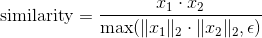
class torch.nn.CosineSimilarity(dim=1, eps=1e-08)

返回沿着 dim 方向计算的 x1 与 x2 之间的余弦相似度.

$\text{similarity} = \dfrac{x_1 \cdot x_2}{\max(\Vert x_1 \Vert _2 \cdot \Vert x_2 \Vert _2, \epsilon)}$

参数：

dim (int, 可选) – 计算余弦相似度的维度. Default: 1
eps (float, 可选) – 小的值以避免被零除. Default: 1e-8

形状：

Input1: $(\ast_1, D, \ast_2)$ , 其中的 D 表示 dim 的位置
Input2: $(\ast_1, D, \ast_2)$ , 与 Input1 一样的 shape
输出： $(\ast_1, \ast_2)$

Examples:

>>> input1 = autograd.Variable(torch.randn(100, 128))
>>> input2 = autograd.Variable(torch.randn(100, 128))
>>> cos = nn.CosineSimilarity(dim=1, eps=1e-6)
>>> output = cos(input1, input2)
>>> print(output)

PairwiseDistance

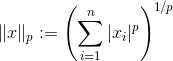
class torch.nn.PairwiseDistance(p=2, eps=1e-06)

计算向量 v1, v2 之间的 batchwise pairwise distance(分批成对距离):

$\Vert x \Vert _p := \left( \sum_{i=1}^n \vert x_i \vert ^ p \right) ^ {1/p}$

参数：

p (_real_) – norm degree(规范程度). Default: 2
eps (float, 可选) – 小的值以避免被零除. Default: 1e-6

形状：

Input1: $(N, D)$ , 其中的 D = vector dimension(向量维度)
Input2: $(N, D)$ , 与 Input1 的 shape 一样
输出： $(N, 1)$

Examples:

>>> pdist = nn.PairwiseDistance(p=2)
>>> input1 = autograd.Variable(torch.randn(100, 128))
>>> input2 = autograd.Variable(torch.randn(100, 128))
>>> output = pdist(input1, input2)

Loss functions (损失函数)

L1Loss

class torch.nn.L1Loss(size_average=True, reduce=True)

创建一个衡量输入 x 与目标 y 之间差的绝对值的平均值的标准, 该函数会逐元素地求出 x 和 y 之间差的绝对值, 最后返回绝对值的平均值.

${loss}(x, y) = 1/n \sum |x_i - y_i|$

x 和 y 可以是任意维度的数组, 但需要有相同数量的n个元素.

求和操作会对n个元素求和, 最后除以 n .

在构造函数的参数中传入 size_average=False, 最后求出来的绝对值将不会除以 n.

参数：

size_average (bool, 可选) – 默认情况下, loss 会在每个 mini-batch(小批量）上取平均值. 如果字段 size_average 被设置为 False, loss 将会在每个 mini-batch(小批量）上累加, 而不会取平均值. 当 reduce 的值为 False 时该字段会被忽略. 默认值: True
reduce (bool, 可选) – 默认情况下, loss 会在每个 mini-batch(小批量）上求平均值或者求和. 当 reduce 是 False 时, 损失函数会对每个 batch 元素都返回一个 loss 并忽略 size_average 字段. 默认值: True

形状：

输入: $(N, *)$ , * 表示任意数量的额外维度
目标: $(N, *)$ , 和输入的shape相同
输出: 标量. 如果 reduce 是 False , 则输出为 $(N, *)$ , shape与输出相同

Examples:

>>> loss = nn.L1Loss()
>>> input = autograd.Variable(torch.randn(3, 5), requires_grad=True)
>>> target = autograd.Variable(torch.randn(3, 5))
>>> output = loss(input, target)
>>> output.backward()

MSELoss

class torch.nn.MSELoss(size_average=True, reduce=True)

输入 x 和目标 y 之间的均方差

${loss}(x, y) = 1/n \sum |x_i - y_i|^2$

x 和 y 可以是任意维度的数组, 但需要有相同数量的n个元素.

求和操作会对n个元素求和, 最后除以 n.

在构造函数的参数中传入 size_average=False , 最后求出来的绝对值将不会除以 n.

要得到每个 batch 中每个元素的 loss, 设置 reduce 为 False. 返回的 loss 将不会取平均值, 也不会被 size_average 影响.

参数：

size_average (bool, 可选) – 默认情况下, loss 会在每个 mini-batch(小批量）上取平均值. 如果字段 size_average 被设置为 False , loss 会在每个 mini-batch(小批量）上求和. 只有当 reduce 的值为 True 才会生效. 默认值: True
reduce (bool, 可选) – 默认情况下, loss 会根据 size_average 的值在每个 mini-batch(小批量）上求平均值或者求和. 当 reduce 是 False 时, 损失函数会对每个 batch 元素都返回一个 loss 并忽略 size_average字段. 默认值: True

形状：

输入: $(N, *)$ , 其中 * 表示任意数量的额外维度.
目标: $(N, *)$ , shape 跟输入相同

Examples:

>>> loss = nn.MSELoss()
>>> input = autograd.Variable(torch.randn(3, 5), requires_grad=True)
>>> target = autograd.Variable(torch.randn(3, 5))
>>> output = loss(input, target)
>>> output.backward()

CrossEntropyLoss

class torch.nn.CrossEntropyLoss(weight=None, size_average=True, ignore_index=-100, reduce=True)

该类把 LogSoftMax 和 NLLLoss 结合到了一个类中

当训练有 C 个类别的分类问题时很有效. 可选参数 weight 必须是一个1维 Tensor, 权重将被分配给各个类别. 对于不平衡的训练集非常有效.

input 含有每个类别的分数

input 必须是一个2维的形如 (minibatch, C) 的 Tensor.

target 是一个类别索引 (0 to C-1), 对应于 minibatch 中的每个元素

loss 可以描述为:

loss(x, class) = -log(exp(x[class]) / (\sum_j exp(x[j])))
               = -x[class] + log(\sum_j exp(x[j]))

当 weight 参数存在时:

loss(x, class) = weight[class] * (-x[class] + log(\sum_j exp(x[j])))

loss 在每个 mini-batch(小批量）上取平均值.

参数：

weight (Tensor, 可选) – 自定义的每个类别的权重. 必须是一个长度为 C 的 Tensor
size_average (bool, 可选) – 默认情况下, loss 会在每个 mini-batch(小批量）上取平均值. 如果字段 size_average 被设置为 False, loss 将会在每个 mini-batch(小批量）上累加, 而不会取平均值. 当 reduce 的值为 False 时该字段会被忽略.
ignore_index (int, 可选) – 设置一个目标值, 该目标值会被忽略, 从而不会影响到输入的梯度. 当 size_average 字段为 True 时, loss 将会在没有被忽略的元素上取平均.
reduce (bool, 可选) – 默认情况下, loss 会根据 size_average 的值在每个 mini-batch(小批量）上求平均值或者求和. 当 reduce 是 False 时, 损失函数会对每个 batch 元素都返回一个 loss 并忽略 size_average 字段. 默认值: True

形状：

输入: $(N, C)$ , 其中 C 是类别的数量
目标: $(N)$ , 其中的每个元素都满足 0 <= targets[i] <= C-1
输出: 标量. 如果 reduce 是 False, 则输出为 $(N)$ .

Examples:

>>> loss = nn.CrossEntropyLoss()
>>> input = autograd.Variable(torch.randn(3, 5), requires_grad=True)
>>> target = autograd.Variable(torch.LongTensor(3).random_(5))
>>> output = loss(input, target)
>>> output.backward()

NLLLoss

class torch.nn.NLLLoss(weight=None, size_average=True, ignore_index=-100, reduce=True)

负对数似然损失. 用于训练 C 个类别的分类问题. 可选参数 weight 是一个1维的 Tensor, 用来设置每个类别的权重. 当训练集不平衡时该参数十分有用.

由前向传播得到的输入应该含有每个类别的对数概率: 输入必须是形如 (minibatch, C) 的 2维 Tensor.

在一个神经网络的最后一层添加 LogSoftmax 层可以得到对数概率. 如果你不希望在神经网络中加入额外的一层, 也可以使用 CrossEntropyLoss 函数.

该损失函数需要的目标值是一个类别索引 (0 到 C-1, 其中 C 是类别数量)

该 loss 可以描述为:

loss(x, class) = -x[class]

或者当 weight 参数存在时可以描述为:

loss(x, class) = -weight[class] * x[class]

又或者当 ignore_index 参数存在时可以描述为:

loss(x, class) = class != ignoreIndex ? -weight[class] * x[class] : 0

参数：

weight (Tensor, 可选) – 自定义的每个类别的权重. 必须是一个长度为 C 的 Tensor
size_average (bool, 可选) – 默认情况下, loss 会在每个 mini-batch(小批量）上取平均值. 如果字段 size_average 被设置为 False, loss 将会在每个 mini-batch(小批量）上累加, 而不会取平均值. 当 reduce 的值为 False 时该字段会被忽略. 默认值: True
ignore_index (int, 可选) – 设置一个目标值, 该目标值会被忽略, 从而不会影响到输入的梯度. 当 size_average 为 True 时, loss 将会在没有被忽略的元素上取平均值.
reduce (bool, 可选) – 默认情况下, loss 会在每个 mini-batch(小批量）上求平均值或者求和. 当 reduce 是 False 时, 损失函数会对每个 batch 元素都返回一个 loss 并忽略 size_average 字段. 默认值: True

形状：

输入: $(N, C)$ , 其中 C 是类别的数量
目标: $(N)$ , 其中的每个元素都满足 0 <= targets[i] <= C-1
输出: 标量. 如果 reduce 是 False, 则输出为 $(N)$ .

Examples:

>>> m = nn.LogSoftmax()
>>> loss = nn.NLLLoss()
>>> # input is of size N x C = 3 x 5
>>> input = autograd.Variable(torch.randn(3, 5), requires_grad=True)
>>> # each element in target has to have 0 <= value < C
>>> target = autograd.Variable(torch.LongTensor([1, 0, 4]))
>>> output = loss(m(input), target)
>>> output.backward()

PoissonNLLLoss

class torch.nn.PoissonNLLLoss(log_input=True, full=False, size_average=True, eps=1e-08)

目标值为泊松分布的负对数似然损失.

该损失可以描述为:

target ~ Pois(input) loss(input, target) = input - target * log(input) + log(target!)

最后一项可以被省略或者用 Stirling 公式来近似. 该近似用于大于1的目标值. 当目标值小于或等于1时, 则将0加到 loss 中.

参数：

log_input (bool, 可选) – 如果设置为 True , loss 将会按照公式 exp(input) - target * input 来计算, 如果设置为 False , loss 将会按照 input - target * log(input+eps) 计算.
full (bool, 可选) – 是否计算全部的 loss, i. e. 加上 Stirling 近似项 target * log(target) - target + 0.5 * log(2 * pi * target).
size_average (bool, 可选) – 默认情况下, loss 会在每个 mini-batch(小批量）上取平均值. 如果字段 size_average 被设置为 False, loss 将会在每个 mini-batch(小批量）上累加, 而不会取平均值.
eps (float, 可选) – 当 log_input==False 时, 取一个很小的值用来避免计算 log(0). 默认值: 1e-8

Examples:

>>> loss = nn.PoissonNLLLoss()
>>> log_input = autograd.Variable(torch.randn(5, 2), requires_grad=True)
>>> target = autograd.Variable(torch.randn(5, 2))
>>> output = loss(log_input, target)
>>> output.backward()

NLLLoss2d

class torch.nn.NLLLoss2d(weight=None, size_average=True, ignore_index=-100, reduce=True)

对于图片输入的负对数似然损失. 它计算每个像素的负对数似然损失.

参数：

weight (Tensor, 可选) – 自定义的每个类别的权重. 必须是一个长度为 C 的 Tensor
size_average – 默认情况下, loss 会在每个 mini-batch(小批量）上取平均值. 如果字段 size_average 被设置为 False, loss 将会在每个 mini-batch(小批量）上累加, 而不会取平均值. 当 reduce 的值为 False 时该字段会被忽略. 默认值: True
reduce (bool, 可选) – 默认情况下, loss 会在每个 mini-batch(小批量）上求平均值或者求和. 当 reduce 是 False 时, 损失函数会对每个 batch 元素都返回一个 loss 并忽略 size_average 字段. 默认值: True

形状：

输入： $(N, C, H, W)$ where C = number of classes
Target: $(N, H, W)$ where each value is 0 <= targets[i] <= C-1
输出：scalar. If reduce is False, then $(N, H, W)$ instead.

Examples:

>>> m = nn.Conv2d(16, 32, (3, 3)).float()
>>> loss = nn.NLLLoss2d()
>>> # input is of size N x C x height x width
>>> input = autograd.Variable(torch.randn(3, 16, 10, 10))
>>> # each element in target has to have 0 <= value < C
>>> target = autograd.Variable(torch.LongTensor(3, 8, 8).random_(0, 4))
>>> output = loss(m(input), target)
>>> output.backward()

KLDivLoss

class torch.nn.KLDivLoss(size_average=True, reduce=True)

Kullback-Leibler divergence 损失

KL 散度可用于衡量不同的连续分布之间的距离, 在连续的输出分布的空间上(离散采样)上进行直接回归时很有效.

跟 NLLLoss 一样, input 需要含有 对数概率 , 不同于 ClassNLLLoss, input 可以不是2维的 Tensor, 因为该函数会逐元素地求值.

该方法需要一个shape跟 input Tensor 一样的 target Tensor.

损失可以描述为:

$loss(x, target) = 1/n \sum(target_i * (log(target_i) - x_i))$

默认情况下, loss 会在每个 mini-batch(小批量）上和维度上取平均值. 如果字段 size_average 设置为 False, 则 loss 不会取平均值.

参数：

size_average (bool, 可选) – 默认情况下, loss 会在每个 mini-batch(小批量）上和维度上取平均值. 如果设置为 False, 则 loss 会累加, 而不是取平均值.
reduce (bool, 可选) – 默认情况下, loss 会根据 size_average 在每个 mini-batch(小批量）上求平均值或者求和. 当 reduce 是 False 时, 损失函数会对每个 batch 元素都返回一个 loss 并忽略 size_average 字段. 默认值: True

形状：

输入: $(N, *)$ , 其中 * 表示任意数量的额外维度.
目标: $(N, *)$ , shape 跟输入相同
输出: 标量. 如果 reduce 是 True, 则输出为 $(N, *)$ , shape 跟输入相同.

BCELoss

class torch.nn.BCELoss(weight=None, size_average=True)

计算目标和输出之间的二进制交叉熵:

$loss(o, t) = - 1/n \sum_i (t[i] * log(o[i]) + (1 - t[i]) * log(1 - o[i]))$

当定义了 weight 参数时:

$loss(o, t) = - 1/n \sum_i weight[i] * (t[i] * log(o[i]) + (1 - t[i]) * log(1 - o[i]))$

这可用于测量重构的误差, 例如自动编码机. 注意目标的值 t[i] 的范围为0到1之间.

参数：

weight (Tensor, 可选) – 自定义的每个 batch 元素的 loss 的权重. 必须是一个长度为 “nbatch” 的的 Tensor
size_average (bool, 可选) – 默认情况下, loss 会在每个 mini-batch(小批量）上取平均值. 如果字段 size_average 被设置为 False , loss 会在每个 mini-batch(小批量）上累加, 而不是取平均值. 默认值: True

形状：

输入: $(N, *)$ , 其中 * 表示任意数量的额外维度.
目标: $(N, *)$ , shape 跟输入相同

Examples:

>>> m = nn.Sigmoid()
>>> loss = nn.BCELoss()
>>> input = autograd.Variable(torch.randn(3), requires_grad=True)
>>> target = autograd.Variable(torch.FloatTensor(3).random_(2))
>>> output = loss(m(input), target)
>>> output.backward()

BCEWithLogitsLoss

class torch.nn.BCEWithLogitsLoss(weight=None, size_average=True)

该损失函数把 Sigmoid 层集成到了 BCELoss 类中. 该版比用一个简单的 Sigmoid 层和 BCELoss 在数值上更稳定, 因为把这两个操作合并为一个层之后, 可以利用 log-sum-exp 的技巧来实现数值稳定.

目标和输出之间的二值交叉熵(不含sigmoid函数)是:

$loss(o, t) = - 1/n \sum_i (t[i] * log(sigmoid(o[i])) + (1 - t[i]) * log(1 - sigmoid(o[i])))$

当定义了 weight 参数之后可描述为:

$loss(o, t) = - 1/n \sum_i weight[i] * (t[i] * log(sigmoid(o[i])) + (1 - t[i]) * log(1 - sigmoid(o[i])))$

这可用于测量重构的误差, 例如自动编码机. 注意目标的值 t[i] 的范围为0到1之间.

参数：

weight (Tensor, 可选) – 自定义的每个 batch 元素的 loss 的权重. 必须是一个长度为 “nbatch” 的 Tensor
size_average (bool, 可选) – 默认情况下, loss 会在每个 mini-batch(小批量）上取平均值. 如果字段 size_average 被设置为 False , loss 会在每个 mini-batch(小批量）上累加, 而不是取平均值. 默认值: True

形状：

输入: $(N, *)$ , 其中 * 表示任意数量的额外维度.
目标: $(N, *)$ , shape 跟输入相同

Examples:

>>> loss = nn.BCEWithLogitsLoss()
>>> input = autograd.Variable(torch.randn(3), requires_grad=True)
>>> target = autograd.Variable(torch.FloatTensor(3).random_(2))
>>> output = loss(input, target)
>>> output.backward()

MarginRankingLoss

class torch.nn.MarginRankingLoss(margin=0, size_average=True)

创建一个衡量 mini-batch(小批量) 中的2个1维 Tensor 的输入 x1 和 x2, 和1个1维 Tensor 的目标 y(y 的取值是 1 或者 -1) 之间损失的标准.

如果 y == 1 则认为第一个输入值应该排列在第二个输入值之上(即值更大), y == -1 时则相反.

对于 mini-batch(小批量) 中每个实例的损失函数如下:

loss(x, y) = max(0, -y * (x1 - x2) + margin)

如果内部变量 size_average = True, 则损失函数计算批次中所有实例的损失值的平均值; 如果 size_average = False, 则损失函数计算批次中所有实例的损失至的合计. size_average 默认值为 True.

HingeEmbeddingLoss

class torch.nn.HingeEmbeddingLoss(margin=1.0, size_average=True)

衡量输入 Tensor(张量) x 和目标 Tensor(张量) y (取值为 1 和 -1) 之间的损失值. 此方法通常用来衡量两个输入值是否相似, 例如使用L1成对距离作为 x, 并且通常用来进行非线性嵌入学习或者半监督学习:

                 { x_i,                  if y_i ==  1
loss(x, y) = 1/n {
                 { max(0, margin - x_i), if y_i == -1

x 和 y 分别可以是具有 n 个元素的任意形状. 合计操作对所有元素进行计算.

如果 size_average=False, 则计算时不会除以 n 取平均值.

margin 的默认值是 1, 或者可以通过构造函数来设置.

MultiLabelMarginLoss

class torch.nn.MultiLabelMarginLoss(size_average=True)

创建一个标准, 用以优化多元分类问题的合页损失函数 (基于空白的损失), 计算损失值时需要2个参数分别为输入, x (一个2维小批量 Tensor) 和输出 y (一个2维 Tensor, 其值为 x 的索引值). 对于mini-batch(小批量) 中的每个样本按如下公式计算损失:

loss(x, y) = sum_ij(max(0, 1 - (x[y[j]] - x[i]))) / x.size(0)

其中 i 的取值范围是 0 到 x.size(0), j 的取值范围是 0 到 y.size(0), y[j] >= 0, 并且对于所有 i 和 j 有 i != y[j].

y 和 x 必须有相同的元素数量.

此标准仅考虑 y[j] 中最先出现的非零值.

如此可以允许每个样本可以有数量不同的目标类别.

SmoothL1Loss

class torch.nn.SmoothL1Loss(size_average=True, reduce=True)

创建一个标准, 当某个元素的错误值的绝对值小于1时使用平方项计算, 其他情况则使用L1范式计算. 此方法创建的标准对于异常值不如 MSELoss敏感, 但是同时在某些情况下可以防止梯度爆炸 (比如参见论文 “Fast R-CNN” 作者 Ross Girshick). 也被称为 Huber 损失函数:

                      { 0.5 * (x_i - y_i)^2, if |x_i - y_i| < 1
loss(x, y) = 1/n \sum {
                      { |x_i - y_i| - 0.5,   otherwise

x 和 y 可以是任意形状只要都具备总计 n 个元素合计仍然针对所有元素进行计算, 并且最后除以 n.

如果把内部变量 size_average 设置为 False, 则不会被除以 n.

参数：

size_average (bool, 可选) – 损失值默认会按照所有元素取平均值. 但是, 如果 size_average 被设置为 False, 则损失值为所有元素的合计. 如果 reduce 参数设为 False, 则忽略此参数的值. 默认: True
reduce (bool, 可选) – 损失值默认会按照所有元素取平均值或者取合计值. 当 reduce 设置为 False 时, 损失函数对于每个元素都返回损失值并且忽略 size_average 参数. 默认: True

形状：

输入: $(N, *)$ * 代表任意个其他维度
目标: $(N, *)$ , 同输入
输出: 标量. 如果 reduce 设为 False 则为 $(N, *)$ , 同输入

SoftMarginLoss

class torch.nn.SoftMarginLoss(size_average=True)

创建一个标准, 用以优化两分类的 logistic loss. 输入为 x (一个2维 mini-batch Tensor)和目标 y (一个包含 1 或者 -1 的 Tensor).

loss(x, y) = sum_i (log(1 + exp(-y[i]*x[i]))) / x.nelement()

可以通过设置 self.size_average 为 False 来禁用按照元素数量取平均的正则化操作.

MultiLabelSoftMarginLoss

class torch.nn.MultiLabelSoftMarginLoss(weight=None, size_average=True)

创建一个标准, 基于输入 x 和目标 y的 max-entropy(最大熵), 优化多标签 one-versus-all 损失. 输入 x 为一个2维 mini-batch Tensor, 目标 y 为2进制2维 Tensor. 对每个 mini-batch 中的样本, 对应的 loss 为:

loss(x, y) = - sum_i (y[i] * log( 1 / (1 + exp(-x[i])))
                  + ( (1-y[i]) * log(exp(-x[i]) / (1 + exp(-x[i]))) )

其中 i == 0 至 x.nElement()-1, y[i] in {0,1}. y 和 x 必须具有相同的维度.

CosineEmbeddingLoss

class torch.nn.CosineEmbeddingLoss(margin=0, size_average=True)

新建一个标准, 用以衡量输入 Tensor x1, x2 和取值为 1 或者 -1 的标签 Tensor y之间的损失值. 此标准用 cosine 距离来衡量2个输入参数之间是否相似, 并且一般用来学习非线性 embedding 或者半监督学习.

margin 应该取 -1 到 1 之间的值, 建议取值范围是 0 到 0.5. 如果没有设置 margin 参数, 则默认值取 0.

每个样本的损失函数如下:

             { 1 - cos(x1, x2),              if y ==  1
loss(x, y) = {
             { max(0, cos(x1, x2) - margin), if y == -1

如果内部变量 size_average 设置为 True, 则损失函数以 batch 中所有的样本数取平均值; 如果 size_average 设置为 False, 则损失函数对 batch 中所有的样本求和. 默认情况下, size_average = True.

MultiMarginLoss

class torch.nn.MultiMarginLoss(p=1, margin=1, weight=None, size_average=True)

创建一个标准, 用以优化多元分类问题的合页损失函数 (基于空白的损失), 计算损失值时需要2个参数分别为输入, x (一个2维小批量 Tensor) 和输出 y (一个1维 Tensor, 其值为 x 的索引值, 0 <= y <= x.size(1)):

对于每个 mini-batch(小批量) 样本:

loss(x, y) = sum_i(max(0, (margin - x[y] + x[i]))^p) / x.size(0)

其中 i == 0 至 x.size(0) 并且 i != y.

可选择的, 如果您不想所有的类拥有同样的权重的话, 您可以通过在构造函数中传入 weight 参数来解决这个问题, weight 是一个1维 Tensor.

传入 weight 后, 损失函数变为:

loss(x, y) = sum_i(max(0, w[y] * (margin - x[y] - x[i]))^p) / x.size(0)

默认情况下, 求出的损失值会对每个 minibatch 样本的结果取平均. 可以通过设置 size_average 为 False 来用合计操作取代取平均操作.

TripletMarginLoss

class torch.nn.TripletMarginLoss(margin=1.0, p=2, eps=1e-06, swap=False)

创建一个标准, 用以衡量三元组合的损失值, 计算损失值时需要3个输入张量 x1, x2, x3 和一个大于零的 margin 值. 此标准可以用来衡量输入样本间的相对相似性. 一个三元输入组合由 a, p 和 n: anchor, positive 样本和 negative 样本组成. 所有输入变量的形式必须为 $(N, D)$ .

距离交换的详细说明请参考论文 Learning shallow convolutional feature descriptors with triplet losses by V. Balntas, E. Riba et al.

$L(a, p, n) = \frac{1}{N} \left( \sum_{i=1}^N \max \{d(a_i, p_i) - d(a_i, n_i) + {\rm margin}, 0\} \right)$

其中 $d(x_i, y_i) = \left\lVert {\bf x}_i - {\bf y}_i \right\rVert_p$ .

参数：

anchor – anchor 输入 tensor
positive – positive 输入 tensor
negative – negative 输入 tensor
p – 正则化率. Default: 2

形状：

输入： $(N, D)$ 其中 D = vector dimension
输出： $(N, 1)$

>>> triplet_loss = nn.TripletMarginLoss(margin=1.0, p=2)
>>> input1 = autograd.Variable(torch.randn(100, 128))
>>> input2 = autograd.Variable(torch.randn(100, 128))
>>> input3 = autograd.Variable(torch.randn(100, 128))
>>> output = triplet_loss(input1, input2, input3)
>>> output.backward()

Vision layers (视觉层)

PixelShuffle

class torch.nn.PixelShuffle(upscale_factor)

对张量中形如 $(*, C * r^2, H, W]$ 的元素, 重新排列成 $(C, H * r, W * r)$ .

当使用 stride = $1/r$ 的高效子像素卷积很有用.

参考如下论文获得更多信息: Real-Time Single Image and Video Super-Resolution Using an Efficient Sub-Pixel Convolutional Neural Network Shi et. al (2016) .

参数：upscale_factor (int) – 增加空间分辨率的因子

形状：

输入: $(N, C * {upscale\_factor}^2, H, W)$
输出: $(N, C, H * {upscale\_factor}, W * {upscale\_factor})$

Examples:

>>> ps = nn.PixelShuffle(3)
>>> input = autograd.Variable(torch.Tensor(1, 9, 4, 4))
>>> output = ps(input)
>>> print(output.size())
torch.Size([1, 1, 12, 12])

Upsample

class torch.nn.Upsample(size=None, scale_factor=None, mode='nearest')

对给定的多通道一维时序数据, 二维空间数据, 或三维容积数据进行上采样.

输入数据的格式为 minibatch x channels x [depth] x [height] x width. 因此, 对于2-D空间数据的输入, 期望得到一个4-D张量；对于3-D立体数据输入, 期望得到一个5-D张量.

对3D, 4D, 5D的输入张量进行最近邻、线性、双线性和三线性采样, 可用于该上采样方法.

可以提供 scale_factor 或目标输出的 size 来计算输出的大小. (不能同时都给, 因为这样做是含糊不清的. )

参数：

size (tuple, 可选) – 整型数的元组 ([D_out], [H_out], W_out) 输出大小
scale_factor (int / tuple[int...], 可选) – 图像高度/宽度/深度的乘数
mode (string, 可选) – 上采样算法: nearest | linear | bilinear | trilinear. 默认为: nearest

形状：

输入: $(N, C, W_{in})$ , $(N, C, H_{in}, W_{in})$ 或 $(N, C, D_{in}, H_{in}, W_{in})$
输出: $(N, C, W_{out})$ , $(N, C, H_{out}, W_{out})$ 或 $(N, C, D_{out}, H_{out}, W_{out})$ 其中: $D_{out} = floor(D_{in} * scale\_factor)$ 或 size[-3] $H_{out} = floor(H_{in} * scale\_factor)$ 或 size[-2] $W_{out} = floor(W_{in} * scale\_factor)$ 或 size[-1]

示例:

>>> inp
Variable containing:
(0 ,0 ,.,.) =
 1  2
 3  4
[torch.FloatTensor of size 1x1x2x2]
>>> m = nn.Upsample(scale_factor=2, mode='bilinear')
>>> m(inp)
Variable containing:
(0 ,0 ,.,.) =
 1.0000  1.3333  1.6667  2.0000
 1.6667  2.0000  2.3333  2.6667
 2.3333  2.6667  3.0000  3.3333
 3.0000  3.3333  3.6667  4.0000
[torch.FloatTensor of size 1x1x4x4]
>>> inp
Variable containing:
(0 ,0 ,.,.) =
 1  2
 3  4
[torch.FloatTensor of size 1x1x2x2]
>>> m = nn.Upsample(scale_factor=2, mode='nearest')
>>> m(inp)
Variable containing:
(0 ,0 ,.,.) =
 1  1  2  2
 1  1  2  2
 3  3  4  4
 3  3  4  4
[torch.FloatTensor of size 1x1x4x4]

UpsamplingNearest2d

class torch.nn.UpsamplingNearest2d(size=None, scale_factor=None)

对多个输入通道组成的输入信号进行2维最近邻上采样.

为了指定采样范围, 提供了 size 或 scale_factor 作为构造参数.

当给定 size, 输出图像的大小为 (h, w).

参数：

size (tuple, 可选) – 输出图片大小的整型元组(H_out, W_out)
scale_factor (int, 可选) – 图像的长和宽的乘子.

形状：

输入： $(N, C, H_{in}, W_{in})$
输出： $(N, C, H_{out}, W_{out})$ 其中 $H_{out} = floor(H_{in} * scale\_factor)$ $W_{out} = floor(W_{in} * scale\_factor)$

示例:

>>> inp
Variable containing:
(0 ,0 ,.,.) =
 1  2
 3  4
[torch.FloatTensor of size 1x1x2x2]
>>> m = nn.UpsamplingNearest2d(scale_factor=2)
>>> m(inp)
Variable containing:
(0 ,0 ,.,.) =
 1  1  2  2
 1  1  2  2
 3  3  4  4
 3  3  4  4
[torch.FloatTensor of size 1x1x4x4]

UpsamplingBilinear2d

class torch.nn.UpsamplingBilinear2d(size=None, scale_factor=None)

对多个输入通道组成的输入信号进行2维双线性上采样.

为了指定采样范围, 提供了 size 或 scale_factor 作为构造参数.

当给定 size, 输出图像的大小为 (h, w).

参数：

size (tuple, 可选) – 输出图片大小的整型元组(H_out, W_out)
scale_factor (int, 可选) – 图像的长和宽的乘子.

形状：

输入： $(N, C, H_{in}, W_{in})$
输出： $(N, C, H_{out}, W_{out})$ 其中 $H_{out} = floor(H_{in} * scale\_factor)$ $W_{out} = floor(W_{in} * scale\_factor)$

示例：

>>> inp
Variable containing:
(0 ,0 ,.,.) =
 1  2
 3  4
[torch.FloatTensor of size 1x1x2x2]
>>> m = nn.UpsamplingBilinear2d(scale_factor=2)
>>> m(inp)
Variable containing:
(0 ,0 ,.,.) =
 1.0000  1.3333  1.6667  2.0000
 1.6667  2.0000  2.3333  2.6667
 2.3333  2.6667  3.0000  3.3333
 3.0000  3.3333  3.6667  4.0000
[torch.FloatTensor of size 1x1x4x4]

DataParallel layers (multi-GPU, distributed) (数据并行层, 多 GPU 的, 分布式的)

DataParallel

class torch.nn.DataParallel(module, device_ids=None, output_device=None, dim=0)

在模块级别实现数据并行性.

此容器通过在批次维度中分块, 将输入分割到指定设备上, 从而并行化给定模块的应用程序.在正向传递中, 模块被复制到每个设备上, 每个副本处理一部分输入.在向后传递期间, 来自每个副本的梯度变化被汇总到原始模块中.

batch size 应该大于 GPUs 的数量.同时也应该是 GPU 数量的整数倍, 以便每个块大小相同(以便每个 GPU 处理相同数量的样本）.

引用 :使用 nn.DataParallel 替代 multiprocessing

允许将任意位置和关键字输入传入 DataParallel EXCEPT Tensors. 所有的变量将被分散在指定的维度(默认为0）.原始类型将被广播, 但所有其他类型将是一个浅层副本, 如果写入模型的正向传递, 可能会被损坏.

Args : module: 并行的模型 device_ids: CUDA devices(CUDA 驱动） (default: all devices) output_device: 输出设备位置 (default: device_ids[0]) 示例 ::

>>> net = torch.nn.DataParallel(model, device_ids=[0, 1, 2])
>>> output = net(input_var)

DistributedDataParallel

class torch.nn.parallel.DistributedDataParallel(module, device_ids=None, output_device=None, dim=0)

在模块级别实现分布式数据并行.

此容器通过在批次维度中分块, 将输入分割到指定设备上, 从而并行化给定模块的应用程序. 该模块被复制到每台机器和每个设备上, 每个这样的副本处理一部分输入.在向后传递期间, 来自每个节点的梯度被平均.

batch size 应该大于 GPUs 的数量.同时也应该是 GPU 数量的整数倍, 以便每个块大小相同(以便每个 GPU 处理相同数量的样本）.

引用 :Basics](distributed.html#distributed-basics) 和使用 nn.DataParallel 替代 multiprocessing. 对输入的约束和 [torch.nn.DataParallel 中一样.

创建这个类需要分布式包已经在 process group 模式下被初始化 (引用 torch.distributed.init_process_group()).

警告：

这个模块只能和gloo后端一起工作.

警告：

构造器, 转发方法和输出(或者这个模块的输出功能）的区分是分布式同步点.考虑到不同的进程可能会执行不同的代码.

警告：

该模块假设所有参数在创建时都在模型中注册.之后不应该添加或删除参数.同样适用于缓冲区.

警告：

这个模块假定所有的缓冲区和梯度都是密集的.

警告：

这个模块不能用于 : func: torch.autograd.grad (即只有在参数的 .grad 属性中累积梯度才能使用）.

注解：

参数永远不会在进程之间广播.模块在梯度上执行全部优化步骤, 并假定它们将以相同的方式在所有进程中进行优化.缓冲区(e.g. BatchNorm stats）在等级0的过程中从模块广播到系统中的每个迭代中的所有其他副本.

Args : module: 需要并行的模型 device_ids: CUDA devices (default: all devices) output_device: device location of output (default: device_ids[0]) 示例 ::

>>> torch.distributed.init_process_group(world_size=4, init_method='...')
>>> net = torch.nn.DistributedDataParallel(model)

Utilities (工具包)

clip_grad_norm

torch.nn.utils.clip_grad_norm(parameters, max_norm, norm_type=2)

接收一个包含 Variable 的可迭代对象, 对 Variable 的梯度按范数进行裁剪.

范数是对所有梯度进行计算的, 等价于把所有输入变量的梯度连接成一个向量, 然后对这个向量按范数进行裁剪. 梯度将会被原地修改.

参数：

parameters (Iterable[Variable]) – 一个可迭代对象, 其包含将要进行梯度正规化的 Variable
max_norm (float 或 int) – 梯度的最大范数
norm_type (float 或 int) – p 范数(指定 p ). 用 'inf' 表示无穷范数

返回值：梯度的范数 (视为单个向量的).

weight_norm

torch.nn.utils.weight_norm(module, name='weight', dim=0)

将权重归一化应用于给定模块中的指定参数. .

$\mathbf{w} = g \dfrac{\mathbf{v}}{\|\mathbf{v}\|}$

权重归一化是将权重张量的大小和方向分离的再参数化. 该函数会用两个参数代替 name (e.g. “weight”)所指定的参数. 在新的参数中, 一个指定参数的大小 (e.g. “weight_g”), 一个指定参数的方向. 权重归一化是通过一个钩子实现的, 该钩子会在 ~Module.forward 的每次调用之前根据大小和方向(两个新参数)重新计算权重张量.

默认情况下, dim=0, 范数会在每一个输出的 channel/plane 上分别计算. 若要对整个权重张量计算范数, 使用 dim=None.

参见 https://arxiv.org/abs/1602.07868

参数：

module (nn.Module) – 给定的 module
name (str, 可选) – 权重参数的 name
dim (int, 可选) – 进行范数计算的维度

返回值：添加了权重归一化钩子的原 module

示例：

>>> m = weight_norm(nn.Linear(20, 40), name='weight')
Linear (20 -> 40)
>>> m.weight_g.size()
torch.Size([40, 1])
>>> m.weight_v.size()
torch.Size([40, 20])

remove_weight_norm

torch.nn.utils.remove_weight_norm(module, name='weight')

从模块中移除权重归一化/再参数化.

参数：

module (nn.Module) – 给定的 module
name (str, 可选) – 权重参数的 name

示例：

>>> m = weight_norm(nn.Linear(20, 40))
>>> remove_weight_norm(m)

PackedSequence

torch.nn.utils.rnn.PackedSequence(_cls, data, batch_sizes)

保存一个打包序列的 data 和 batch_sizes.

所有的 RNN 模块都接收这种被包裹后的序列作为它们的输入.

注解：

永远不要手动创建这个类的实例. 它们应当被 pack_padded_sequence() 这样的函数实例化.

变量：

data (Variable) – 包含打包后序列的 Variable
batch_sizes (list[int]) – 包含每个序列步的 batch size 的列表

pack_padded_sequence

torch.nn.utils.rnn.pack_padded_sequence(input, lengths, batch_first=False)

将填充过的变长序列打包(压紧).

输入的形状可以是 TxBx* . T是最长序列长度(等于 lengths[0]), B是批量大小, *代表任意维度(可以是 0). 如果 batch_first=True , 那么相应的输入大小就是 BxTx* .

Variable 中保存的序列, 应该按序列长度的长短排序, 长的在前, 短的在后. 即 input[:,0] 代表的是最长的序列, input[:, B-1] 保存的是最短的序列.

注解：

只要是维度大于等于2的 input 都可以作为这个函数的参数. 你可以用它来打包 labels, 然后用 RNN 的输出和打包后的 labels 来计算 loss. 通过 PackedSequence 对象的 .data 属性可以获取 Variable.

参数：

input (Variable) – 变长序列被填充后的 batch
lengths (list[int]) – Variable 中每个序列的长度.
batch_first (bool, 可选) – 如果是 True, input 的形状应该是 BxTx*.

返回值：一个 PackedSequence 对象.

pad_packed_sequence

torch.nn.utils.rnn.pad_packed_sequence(sequence, batch_first=False, padding_value=0.0)

填充打包过的变长序列.

这是 pack_padded_sequence() 的逆操作.

返回的 Varaible 的值的 size 是 TxBx*, T 是最长序列的长度, B 是 batch_size, 如果 batch_first=True, 那么返回值是 BxTx*.

Batch中的元素将会以它们长度的逆序排列.

参数：

sequence (PackedSequence) – 将要被填充的 batch
batch_first (bool, 可选) – 如果为 True , 返回的数据的格式为 BxTx*.
padding_value (float, 可选) – 用来填充元素的值

返回值：一个 tuple, 包含被填充后的序列, 和 batch 中序列的长度列表.