本篇笔记以介绍 pytorch 中的 autograd 模块功能为主,主要涉及 torch/autograd 下代码,不涉及底层的 C++ 实现。本文涉及的源码以 PyTorch 1.7 为准。
torch.autograd.function (函数的反向传播)
我们在构建网络的时候,通常使用 pytorch 所提供的nn.Module (例如nn.Conv2d, nn.ReLU等)作为基本单元。而这些 Module 通常是包裹 autograd function,以其作为真正实现的部分。例如nn.ReLU 实际使用torch.nn.functional.relu(F.relu):
from torch.nn import functional as Fclass ReLU(Module):__constants__ = ['inplace']inplace: booldef __init__(self, inplace: bool = False):super(ReLU, self).__init__()self.inplace = inplacedef forward(self, input: Tensor) -> Tensor:return F.relu(input, inplace=self.inplace)
这里的F.relu类型为function,若再剥开一层,其实际包裹的函数类型为builtin_function_or_method,这也是真正完成运算的部分。这些部分通常使用 C++ 实现(如ATen)。至此我们知道,一个模型的运算部分由 autograd functions 组成,这些 autograd functions 内部定义了 forward,backward 用以描述前向和梯度反传的过程,组合后可以实现整个模型的前向和梯度反传。以torch.autograd.function中所定义的Function类为基类,我们可以实现自定义的autograd function,所实现的 function 需包含forward及backward两个方法。以下以Exp和GradCoeff两个自定义 autograd function 为例进行讲解:
class Exp(Function):                    # 此层计算e^x

    @staticmethod
    def forward(ctx, i):                # 模型前向
        result = i.exp()
        ctx.save_for_backward(result)   # 保存所需内容,以备backward时使用,所需的结果会被保存在saved_tensors元组中;此处仅能保存tensor类型变量,若其余类型变量(Int等),可直接赋予ctx作为成员变量,也可以达到保存效果
        return result

    @staticmethod
    def backward(ctx, grad_output):     # 模型梯度反传
        result, = ctx.saved_tensors     # 取出forward中保存的result
        return grad_output * result     # 计算梯度并返回

# 尝试使用
x = torch.tensor([1.], requires_grad=True)  # 需要设置tensor的requires_grad属性为True,才会进行梯度反传
ret = Exp.apply(x)                          # 使用apply方法调用自定义autograd function
print(ret)                                  # tensor([2.7183], grad_fn=<ExpBackward>)
ret.backward()                              # 反传梯度
print(x.grad)                               # tensor([2.7183])
Exp 函数的前向很简单,直接调用 tensor 的成员方法exp即可。反向时,我们知道 , 因此我们直接使用
  乘以
乘以grad_output即得梯度。我们发现,我们自定义的函数Exp正确地进行了前向与反向。同时我们还注意到,前向后所得的结果包含了grad_fn属性,这一属性指向用于计算其梯度的函数(即Exp的backward函数)。关于这点,在接下来的部分会有更详细的说明。接下来我们看另一个函数GradCoeff,其功能是反传梯度时乘以一个自定义系数。
class GradCoeff(Function):

    @staticmethod
    def forward(ctx, x, coeff):                 # 模型前向
        ctx.coeff = coeff                       # 将coeff存为ctx的成员变量
        return x.view_as(x)

    @staticmethod
    def backward(ctx, grad_output):             # 模型梯度反传
        return ctx.coeff * grad_output, None    # backward的输出个数,应与forward的输入个数相同,此处coeff不需要梯度,因此返回None

# 尝试使用
x = torch.tensor([2.], requires_grad=True)
ret = GradCoeff.apply(x, -0.1)                  # 前向需要同时提供x及coeff,设置coeff为-0.1
ret = ret ** 2
print(ret)                                      # tensor([4.], grad_fn=<PowBackward0>)
ret.backward()
print(x.grad)
torch.autograd.functional (计算图的反向传播)
在此前一节,我们描述了单个函数的反向传播,以及如何编写定制的 autograd function。在这一节中,我们简单介绍 pytorch 中所提供的计算图反向传播的接口。
在训练过程中,我们通常利用 prediction 和 groundtruth label 来计算 loss(loss 的类型为Tensor),随后调用loss.backward()进行梯度反传。而 Tensor 类的backward方法,实际调用的就是torch.autograd.backward这一接口。这一 python 接口实现了计算图级的反向传播。
[torch/tensor.py]
class Tensor(torch._C._TensorBase)

    def backward(self, gradient=None, retain_graph=None, create_graph=False):
        relevant_args = (self,)
        ...
        torch.autograd.backward(self, gradient, retain_graph, create_graph)
        # gradient: 形状与tensor一致,可以理解为链式求导的中间结果,若tensor标量,可以省略(默认为1)
        # retain_graph: 多次反向传播时梯度累加。反向传播的中间缓存会被清空,为进行多次反向传播需指定retain_graph=True来保存这些缓存。
        # create_graph: 为反向传播的过程同样建立计算图,可用于计算二阶导
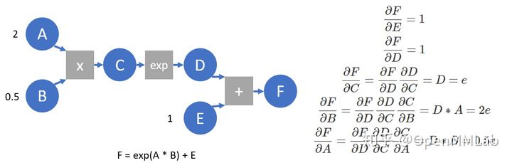
在 pytorch 实现中,autograd 会随着用户的操作,记录生成当前 variable 的所有操作,并建立一个有向无环图 (DAG)。图中记录了操作Function,每一个变量在图中的位置可通过其grad_fn属性在图中的位置推测得到。在反向传播过程中,autograd 沿着这个图从当前变量(根节点 F)溯源,可以利用链式求导法则计算所有叶子节点的梯度。每一个前向传播操作的函数都有与之对应的反向传播函数用来计算输入的各个 variable 的梯度,这些函数的函数名通常以Backward结尾。我们构建一个简化的计算图,并以此为例进行简单介绍。
A = torch.tensor(2., requires_grad=True)
B = torch.tensor(.5, requires_grad=True)
E = torch.tensor(1., requires_grad=True)
C = A * B
D = C.exp()
F = D + E
print(F)        # tensor(3.7183, grad_fn=<AddBackward0>) 打印计算结果,可以看到F的grad_fn指向AddBackward,即产生F的运算
print([x.is_leaf for x in [A, B, C, D, E, F]])  # [True, True, False, False, True, False] 打印是否为叶节点,由用户创建,且requires_grad设为True的节点为叶节点
print([x.grad_fn for x in [F, D, C, A]])    # [<AddBackward0 object at 0x7f972de8c7b8>, <ExpBackward object at 0x7f972de8c278>, <MulBackward0 object at 0x7f972de8c2b0>, None]  每个变量的grad_fn指向产生其算子的backward function,叶节点的grad_fn为空
print(F.grad_fn.next_functions) # ((<ExpBackward object at 0x7f972de8c390>, 0), (<AccumulateGrad object at 0x7f972de8c5f8>, 0)) 由于F = D + E, 因此F.grad_fn.next_functions也存在两项,分别对应于D, E两个变量,每个元组中的第一项对应于相应变量的grad_fn,第二项指示相应变量是产生其op的第几个输出。E作为叶节点,其上没有grad_fn,但有梯度累积函数,即AccumulateGrad(由于反传时多出可能产生梯度,需要进行累加)
F.backward(retain_graph=True)   # 进行梯度反传
print(A.grad, B.grad, E.grad)   # tensor(1.3591) tensor(5.4366) tensor(1.) 算得每个变量梯度,与求导得到的相符
print(C.grad, D.grad)   # None None 为节约空间,梯度反传完成后,中间节点的梯度并不会保留
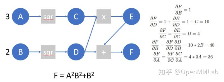
我们再来看下面的计算图,并在这个计算图上模拟 autograd 所做的工作:
A = torch.tensor([3.], requires_grad=True)
B = torch.tensor([2.], requires_grad=True)
C = A ** 2
D = B ** 2
E = C * D
F = D + E

F.manual_grad = torch.tensor(1)                             # 我们用manual_grad表示,在已知计算图结构的情况下,我们模拟autograd过程手动算得的梯度
D.manual_grad, E.manual_grad = F.grad_fn(F.manual_grad)
C.manual_grad, tmp2 = E.grad_fn(E.manual_grad)
D.manual_grad = D.manual_grad + tmp2                        # 这里我们先完成D上的梯度累加,再进行反传
A.manual_grad = C.grad_fn(C.manual_grad)
B.manual_grad = D.grad_fn(D.manual_grad)                    # (tensor([24.], grad_fn=<MulBackward0>), tensor([40.], grad_fn=<MulBackward0>))
下面,我们编写一个简单的函数,在这个计算图上进行autograd,并验证结果是否正确:
# 这一例子仅可用于每个op只产生一个输出的情况,且效率很低(由于对于某一节点,每次未等待所有梯度反传至此节点,就直接将本次反传回的梯度直接反传至叶节点)
def autograd(grad_fn, gradient):
    auto_grad = {}
    queue = [[grad_fn, gradient]]
    while queue != []:
        item = queue.pop()
        gradients = item[0](item[1])
        functions = [x[0] for x in item[0].next_functions]
        if type(gradients) is not tuple:
            gradients = (gradients, )
        for grad, func in zip(gradients, functions):
            """叶节点,其上没有grad_fn,但有梯度累积函数,即AccumulateGrad
            Every time a variable is back propogated through,
            the gradient will be accumulated instead of being replaced.
            (This makes it easier for rnn, because each module will
            be back propogated through several times.)
            """
            if type(func).__name__ == 'AccumulateGrad':
                if hasattr(func.variable, 'auto_grad'):
                    func.variable.auto_grad = func.variable.auto_grad + grad
                else:
                    func.variable.auto_grad = grad
            else:
                queue.append([func, grad])

A = torch.tensor([3.], requires_grad=True)
B = torch.tensor([2.], requires_grad=True)
C = A ** 2
D = B ** 2
E = C * D
F = D + E

autograd(F.grad_fn, torch.tensor(1))
print(A.auto_grad, B.auto_grad)         # tensor(24., grad_fn=<UnbindBackward>) tensor(40., grad_fn=<AddBackward0>)

# 这一autograd同样可作用于编写的模型,我们将会看到,它与pytorch自带的backward产生了同样的结果
from torch import nn

class MLP(nn.Module):
    def __init__(self):
        super().__init__()
        self.fc1 = nn.Linear(10, 5)
        self.relu = nn.ReLU()
        self.fc2 = nn.Linear(5, 2)
        self.fc3 = nn.Linear(5, 2)
        self.fc4 = nn.Linear(2, 2)

    def forward(self, x):
        x = self.fc1(x)
        x = self.relu(x)
        x1 = self.fc2(x)
        x2 = self.fc3(x)
        x2 = self.relu(x2)
        x2 = self.fc4(x2)
        return x1 + x2

x = torch.ones([10], requires_grad=True)
mlp = MLP()
mlp_state_dict = mlp.state_dict()

# 自定义autograd
mlp = MLP()
mlp.load_state_dict(mlp_state_dict)
y = mlp(x)
z = torch.sum(y)
autograd(z.grad_fn, torch.tensor(1.))
print(x.auto_grad) # tensor([-0.0121,  0.0055, -0.0756, -0.0747,  0.0134,  0.0867, -0.0546,  0.1121, -0.0934, -0.1046], grad_fn=<AddBackward0>)

mlp = MLP()
mlp.load_state_dict(mlp_state_dict)
y = mlp(x)
z = torch.sum(y)
z.backward()
print(x.grad) # tensor([-0.0121,  0.0055, -0.0756, -0.0747,  0.0134,  0.0867, -0.0546,  0.1121, -0.0934, -0.1046])
pytorch 使用动态图,它的计算图在每次前向传播时都是从头开始构建,所以它能够使用python 控制语句(如 for、if 等)根据需求创建计算图。下面提供一个例子:
def f(x):
    result = 1
    for ii in x:
        if ii.item()>0: result=ii*result
    return result

x = torch.tensor([0.3071,  1.1043,  1.3605, -0.3471], requires_grad=True)
y = f(x)    # y = x[0]*x[1]*x[2]
y.backward()
print(x.grad)   # tensor([1.5023, 0.4178, 0.3391, 0.0000])

x = torch.tensor([ 1.2817,  1.7840, -1.7033,  0.1302], requires_grad=True)
y = f(x)    # y = x[0]*x[1]*x[3]
y.backward()
print(x.grad)   # tensor([0.2323, 0.1669, 0.0000, 2.2866])
此前的例子使用的是Tensor.backward()接口(内部调用autograd.backward),下面我们来介绍autograd提供的jacobian()和hessian()接口,并直接利用其进行自动微分。这两个函数的输入为运算函数(接受输入 tensor,返回输出 tensor)和输入 tensor,返回 jacobian 和 hessian 矩阵。对于jacobian接口,输入输出均可以为 n 维张量,对于hessian接口,输出必需为一标量。jacobian返回的张量 shape 为output_dim x input_dim(若函数输出为标量,则 output_dim 可省略),hessian返回的张量为input_dim x input_dim。除此之外,这两个自动微分接口同时支持运算函数接收和输出多个 tensor。
from torch.autograd.functional import jacobian, hessian
from torch.nn import Linear, AvgPool2d

fc = Linear(4, 2)
pool = AvgPool2d(kernel_size=2)

def scalar_func(x):
    y = x ** 2
    z = torch.sum(y)
    return z

def vector_func(x):
    y = fc(x)
    return y

def mat_func(x):
    x = x.reshape((1, 1,) + x.shape)
    x = pool(x)
    x = x.reshape(x.shape[2:])
    return x ** 2

vector_input = torch.randn(4, requires_grad=True)
mat_input = torch.randn((4, 4), requires_grad=True)

j = jacobian(scalar_func, vector_input)
assert j.shape == (4, )
assert torch.all(jacobian(scalar_func, vector_input) == 2 * vector_input)
h = hessian(scalar_func, vector_input)
assert h.shape == (4, 4)
assert torch.all(hessian(scalar_func, vector_input) == 2 * torch.eye(4))
j = jacobian(vector_func, vector_input)
assert j.shape == (2, 4)
assert torch.all(j == fc.weight)
j = jacobian(mat_func, mat_input)
assert j.shape == (2, 2, 4, 4)
在此前的例子中,我们已经介绍了,autograd.backward()为节约空间,仅会保存叶节点的梯度。若我们想得知输出关于某一中间结果的梯度,我们可以选择使用autograd.grad()接口,或是使用hook机制:
A = torch.tensor(2., requires_grad=True)
B = torch.tensor(.5, requires_grad=True)
C = A * B
D = C.exp()
torch.autograd.grad(D, (C, A))  # (tensor(2.7183), tensor(1.3591)), 返回的梯度为tuple类型, grad接口支持对多个变量计算梯度

def variable_hook(grad):                        # hook注册在Tensor上,输入为反传至这一tensor的梯度
    print('the gradient of C is:', grad)

A = torch.tensor(2., requires_grad=True)
B = torch.tensor(.5, requires_grad=True)
C = A * B
hook_handle = C.register_hook(variable_hook)    # 在中间变量C上注册hook
D = C.exp()
D.backward()                                    # 反传时打印:the gradient of C is: tensor(2.7183)
hook_handle.remove()                            # 如不再需要,可remove掉这一hook
torch.autograd.gradcheck (数值梯度检查)
在编写好自己的 autograd function 后,可以利用gradcheck中提供的gradcheck和gradgradcheck接口,对数值算得的梯度和求导算得的梯度进行比较,以检查backward是否编写正确。以函数  为例,数值法求得
  点的梯度为:
  。 在下面的例子中,我们自己实现了
Sigmoid函数,并利用gradcheck来检查backward的编写是否正确。
class Sigmoid(Function):

    @staticmethod
    def forward(ctx, x):
        output = 1 / (1 + torch.exp(-x))
        ctx.save_for_backward(output)
        return output

    @staticmethod
    def backward(ctx, grad_output):
        output,  = ctx.saved_tensors
        grad_x = output * (1 - output) * grad_output
        return grad_x


test_input = torch.randn(4, requires_grad=True)     # tensor([-0.4646, -0.4403,  1.2525, -0.5953], requires_grad=True)
torch.autograd.gradcheck(Sigmoid.apply, (test_input,), eps=1e-3)    # pass
torch.autograd.gradcheck(torch.sigmoid, (test_input,), eps=1e-3)    # pass
torch.autograd.gradcheck(Sigmoid.apply, (test_input,), eps=1e-4)    # fail
torch.autograd.gradcheck(torch.sigmoid, (test_input,), eps=1e-4)    # fail
我们发现:eps 为 1e-3 时,我们编写的 Sigmoid 和 torch 自带的 builtin Sigmoid 都可以通过梯度检查,但 eps 下降至 1e-4 时,两者反而都无法通过。而一般直觉下,计算数值梯度时, eps 越小,求得的值应该更接近于真实的梯度。这里的反常现象,是由于机器精度带来的误差所致:test_input的类型为torch.float32,因此在 eps 过小的情况下,产生了较大的精度误差(计算数值梯度时,eps 作为被除数),因而与真实精度间产生了较大的 gap。将test_input换为float64的 tensor 后,不再出现这一现象。这点同时提醒我们,在编写backward时,要考虑的数值计算的一些性质,尽可能保留更精确的结果。
test_input = torch.randn(4, requires_grad=True, dtype=torch.float64)    # tensor([-0.4646, -0.4403,  1.2525, -0.5953], dtype=torch.float64, requires_grad=True)
torch.autograd.gradcheck(Sigmoid.apply, (test_input,), eps=1e-4)    # pass
torch.autograd.gradcheck(torch.sigmoid, (test_input,), eps=1e-4)    # pass

torch.autograd.gradcheck(Sigmoid.apply, (test_input,), eps=1e-6)    # pass
torch.autograd.gradcheck(torch.sigmoid, (test_input,), eps=1e-6)    # pass
torch.autograd.anomaly_mode (在自动求导时检测错误产生路径)
可用于在自动求导时检测错误产生路径,借助with autograd.detect_anomaly(): 或是 torch.autograd.set_detect_anomaly(True)来启用:
>>> import torch
>>> from torch import autograd
>>>
>>> class MyFunc(autograd.Function):
...
...     @staticmethod
...     def forward(ctx, inp):
...         return inp.clone()
...
...     @staticmethod
...     def backward(ctx, gO):
...         # Error during the backward pass
...         raise RuntimeError("Some error in backward")
...         return gO.clone()
>>>
>>> def run_fn(a):
...     out = MyFunc.apply(a)
...     return out.sum()
>>>
>>> inp = torch.rand(10, 10, requires_grad=True)
>>> out = run_fn(inp)
>>> out.backward()
    Traceback (most recent call last):
      Some Error Log
    RuntimeError: Some error in backward
>>> with autograd.detect_anomaly():
...     inp = torch.rand(10, 10, requires_grad=True)
...     out = run_fn(inp)
...     out.backward()
    Traceback of forward call that caused the error:            # 检测到错误发生的Trace
      File "tmp.py", line 53, in <module>
        out = run_fn(inp)
      File "tmp.py", line 44, in run_fn
        out = MyFunc.apply(a)
    Traceback (most recent call last):
      Some Error Log
    RuntimeError: Some error in backward
torch.autograd.grad_mode (设置是否需要梯度)
我们在 inference 的过程中,不希望 autograd 对 tensor 求导,因为求导需要缓存许多中间结构,增加额外的内存/显存开销。在 inference 时,关闭自动求导可实现一定程度的速度提升,并节省大量内存及显存(被节省的不仅限于原先用于梯度存储的部分)。我们可以利用grad_mode中的troch.no_grad()来关闭自动求导:
from torchvision.models import resnet50
import torch
net = resnet50().cuda(0)
num = 128
inp = torch.ones([num, 3, 224, 224]).cuda(0)
net(inp)                                        # 若不开torch.no_grad(),batch_size为128时就会OOM (在1080 Ti上)
net = resnet50().cuda(1)
num = 512
inp = torch.ones([num, 3, 224, 224]).cuda(1)
with torch.no_grad():                           # 打开torch.no_grad()后,batch_size为512时依然能跑inference (节约超过4倍显存)
    net(inp)
model.eval()与torch.no_grad()
这两项实际无关,在 inference 的过程中需要都打开:model.eval()令 model 中的BatchNorm, Dropout等 module 采用 eval mode,保证 inference 结果的正确性,但不起到节省显存的作用;torch.no_grad()声明不计算梯度,节省大量内存和显存。
torch.autograd.profiler (提供function级别的统计信息)
import torch
from torchvision.models import resnet18

x = torch.randn((1, 3, 224, 224), requires_grad=True)
model = resnet18()
with torch.autograd.profiler.profile() as prof:
    for _ in range(100):
        y = model(x)
        y = torch.sum(y)
        y.backward()
# NOTE: some columns were removed for brevity
print(prof.key_averages().table(sort_by="self_cpu_time_total"))
输出为包含 CPU 时间及占比,调用次数等信息(由于一个 kernel 可能还会调用其他 kernel,因此 Self CPU 指他本身所耗时间(不含其他 kernel 被调用所耗时间)):
---------------------------------------------  ------------  ------------  ------------  ------------  ------------  ------------
                                         Name    Self CPU %      Self CPU   CPU total %     CPU total  CPU time avg    # of Calls
---------------------------------------------  ------------  ------------  ------------  ------------  ------------  ------------
      aten::mkldnn_convolution_backward_input        18.69%        1.722s        18.88%        1.740s     870.001us          2000
                     aten::mkldnn_convolution        17.07%        1.573s        17.28%        1.593s     796.539us          2000
    aten::mkldnn_convolution_backward_weights        16.96%        1.563s        17.21%        1.586s     792.996us          2000
                      aten::native_batch_norm         9.51%     876.994ms        15.06%        1.388s     694.049us          2000
                aten::max_pool2d_with_indices         9.47%     872.695ms         9.48%     873.802ms       8.738ms           100
                                 aten::select         7.00%     645.298ms        10.06%     926.831ms       7.356us        126000
             aten::native_batch_norm_backward         6.67%     614.718ms        12.16%        1.121s     560.466us          2000
                             aten::as_strided         3.07%     282.885ms         3.07%     282.885ms       2.229us        126900
                                   aten::add_         2.85%     262.832ms         2.85%     262.832ms      37.350us          7037
                                  aten::empty         1.23%     113.274ms         1.23%     113.274ms       4.089us         27700
                     aten::threshold_backward         1.10%     101.094ms         1.17%     107.383ms      63.166us          1700
                                    aten::add         0.88%      81.476ms         0.99%      91.350ms      32.625us          2800
       aten::max_pool2d_with_indices_backward         0.86%      79.174ms         1.02%      93.706ms     937.064us           100
                             aten::threshold_         0.56%      51.678ms         0.56%      51.678ms      30.399us          1700
              torch::autograd::AccumulateGrad         0.40%      36.909ms         2.81%     258.754ms      41.072us          6300
                             aten::empty_like         0.35%      32.532ms         0.63%      57.630ms       6.861us          8400
                      NativeBatchNormBackward         0.32%      29.572ms        12.48%        1.151s     575.252us          2000
                           aten::_convolution         0.31%      28.182ms        17.63%        1.625s     812.258us          2000
                                     aten::mm         0.27%      24.983ms         0.32%      29.522ms     147.611us           200
                                 aten::stride         0.27%      24.665ms         0.27%      24.665ms       0.583us         42300
            aten::mkldnn_convolution_backward         0.22%      20.025ms        36.33%        3.348s       1.674ms          2000
                    MkldnnConvolutionBackward         0.21%      19.112ms        36.53%        3.367s       1.684ms          2000
                                  aten::relu_         0.20%      18.611ms         0.76%      70.289ms      41.346us          1700
                 aten::_batch_norm_impl_index         0.16%      14.298ms        15.32%        1.413s     706.254us          2000
                                  aten::addmm         0.14%      12.684ms         0.15%      14.138ms     141.377us           100
                                  aten::fill_         0.14%      12.672ms         0.14%      12.672ms      21.120us           600
                                ReluBackward1         0.13%      11.845ms         1.29%     119.228ms      70.134us          1700
                            aten::as_strided_         0.13%      11.674ms         0.13%      11.674ms       1.946us          6000
                                    aten::div         0.11%      10.246ms         0.13%      12.288ms     122.876us           100
                             aten::batch_norm         0.10%       8.894ms        15.42%        1.421s     710.700us          2000
                            aten::convolution         0.08%       7.478ms        17.71%        1.632s     815.997us          2000
                                    aten::sum         0.08%       7.066ms         0.10%       9.424ms      31.415us           300
                                 aten::conv2d         0.07%       6.851ms        17.78%        1.639s     819.423us          2000
                             aten::contiguous         0.06%       5.597ms         0.06%       5.597ms       0.903us          6200
                                  aten::copy_         0.04%       3.759ms         0.04%       3.980ms       7.959us           500
                                      aten::t         0.04%       3.526ms         0.06%       5.561ms      11.122us           500
                                   aten::view         0.03%       2.611ms         0.03%       2.611ms       8.702us           300
                                   aten::div_         0.02%       1.973ms         0.04%       4.051ms      40.512us           100
                                 aten::expand         0.02%       1.720ms         0.02%       2.225ms       7.415us           300
                                AddmmBackward         0.02%       1.601ms         0.37%      34.141ms     341.414us           100
                                     aten::to         0.02%       1.596ms         0.04%       3.871ms      12.902us           300
                                   aten::mean         0.02%       1.485ms         0.10%       9.204ms      92.035us           100
                                 AddBackward0         0.01%       1.381ms         0.01%       1.381ms       1.726us           800
                              aten::transpose         0.01%       1.297ms         0.02%       2.035ms       4.071us           500
                          aten::empty_strided         0.01%       1.163ms         0.01%       1.163ms       3.877us           300
                 MaxPool2DWithIndicesBackward         0.01%       1.095ms         1.03%      94.802ms     948.018us           100
                                MeanBackward1         0.01%     974.822us         0.16%      14.393ms     143.931us           100
                                aten::resize_         0.01%     911.689us         0.01%     911.689us       3.039us           300
                             aten::zeros_like         0.01%     884.496us         0.11%      10.384ms     103.843us           100
                                  aten::clone         0.01%     798.993us         0.04%       3.687ms      18.435us           200
                                aten::reshape         0.01%     763.804us         0.03%       2.604ms      13.021us           200
                                  aten::zero_         0.01%     689.598us         0.13%      11.919ms      59.595us           200
                             aten::resize_as_         0.01%     562.349us         0.01%     776.967us       7.770us           100
                             aten::max_pool2d         0.01%     492.109us         9.49%     874.295ms       8.743ms           100
                    aten::adaptive_avg_pool2d         0.01%     469.736us         0.10%       9.673ms      96.733us           100
                              aten::ones_like         0.00%     460.352us         0.01%       1.377ms      13.766us           100
                                 SumBackward0         0.00%     399.188us         0.01%       1.206ms      12.057us           100
                                aten::flatten         0.00%     397.053us         0.02%       1.917ms      19.165us           100
                                 ViewBackward         0.00%     351.824us         0.02%       1.436ms      14.365us           100
                                    TBackward         0.00%     308.947us         0.01%       1.315ms      13.150us           100
                                       detach         0.00%     127.329us         0.00%     127.329us       2.021us            63
                   torch::autograd::GraphRoot         0.00%     114.731us         0.00%     114.731us       1.147us           100
                                 aten::detach         0.00%     106.170us         0.00%     233.499us       3.706us            63
---------------------------------------------  ------------  ------------  ------------  ------------  ------------  ------------
Self CPU time total: 9.217s

若有收获,就点个赞吧
0 人点赞
