- All Import Statements Defined Here
- Note: Do not add to this list.
- All the dependencies you need, can be installed by running .
- ————————
- ————————
- ——————————————-
- Run This Cell to Produce Your Plot
- ———————————————
- Rescale (normalize) the rows to make them each of unit-length
- —————————
- Write your polysemous word exploration code here.
- —————————
- —————————
- Write your incorrect analogy exploration code here.
- —————————
- 导入包
```python
All Import Statements Defined Here
Note: Do not add to this list.
All the dependencies you need, can be installed by running .
————————
import sys assert sys.version_info[0]==3 assert sys.version_info[1] >= 5
from gensim.models import KeyedVectors from gensim.test.utils import datapath import pprint import matplotlib.pyplot as plt plt.rcParams[‘figure.figsize’] = [10, 5] import nltk nltk.download(‘reuters’) from nltk.corpus import reuters import numpy as np import random import scipy as sp from sklearn.decomposition import TruncatedSVD from sklearn.decomposition import PCA
START_TOKEN = ‘
np.random.seed(0) random.seed(0)
————————
<a name="iCCJi"></a># 基于计数的词向量- 读入语料库```pythondef read_corpus(category="crude"):""" Read files from the specified Reuter's category.Params:category (string): category nameReturn:list of lists, with words from each of the processed files"""files = reuters.fileids(category)return [[START_TOKEN] + [w.lower() for w in list(reuters.words(f))] + [END_TOKEN] for f in files]
reuters_corpus = read_corpus()pprint.pprint(reuters_corpus[:3], compact=True, width=100)
将语料库中不同的单词存储在一个 list(corpus_words)中,并计算不同单词总数
def distinct_words(corpus):""" Determine a list of distinct words for the corpus.Params:corpus (list of list of strings): corpus of documentsReturn:corpus_words (list of strings): list of distinct words across the corpus, sorted (using python 'sorted' function)num_corpus_words (integer): number of distinct words across the corpus"""corpus_words = []num_corpus_words = -1# ------------------# Write your implementation here.corpus_words = sorted(list(set([word for words_list in corpus for word in words_list])))num_corpus_words = len(corpus_words)# ------------------return corpus_words, num_corpus_words
计算 co-occurrence matrix(计数的方式)
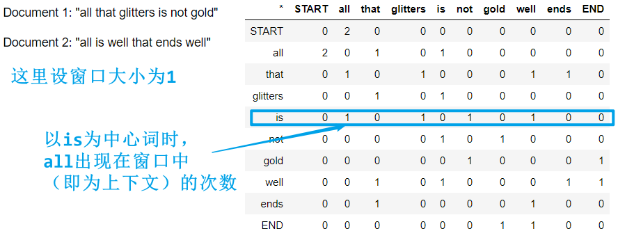
def compute_co_occurrence_matrix(corpus, window_size=4):""" Compute co-occurrence matrix for the given corpus and window_size (default of 4).Note: Each word in a document should be at the center of a window. Words near edges will have a smallernumber of co-occurring words.For example, if we take the document "START All that glitters is not gold END" with window size of 4,"All" will co-occur with "START", "that", "glitters", "is", and "not".Params:corpus (list of list of strings): corpus of documentswindow_size (int): size of context windowReturn:M (numpy matrix of shape (number of corpus words, number of corpus words)):Co-occurence matrix of word counts.The ordering of the words in the rows/columns should be the same as the ordering of the words given by the distinct_words function.word2Ind (dict): dictionary that maps word to index (i.e. row/column number) for matrix M."""words, num_words = distinct_words(corpus)M = Noneword2Ind = {}# ------------------# Write your implementation here.M = np.zeros((num_words, num_words))word2Ind = dict(zip(words, range(num_words)))for doc in corpus:doc_len = len(doc)for current_idx in range(0, doc_len):left_boundary = max(current_idx - window_size, 0)right_boundary = min(current_idx + window_size + 1, doc_len)outside_words = doc[left_boundary : current_idx] + doc[current_idx + 1 : right_boundary]center_word = doc[current_idx]center_idx = word2Ind[center_word]for outside_word in outside_words:outside_idx = word2Ind[outside_word]M[outside_idx, center_idx] += 1# ------------------return M, word2Ind
使用 TruncatedSVD 将 co-occurrence matrix 降维为 k 维
降维后矩阵大小:行数=语料库中不同单词总数,列数=k,即每个单词用 k 维向量表示
def reduce_to_k_dim(M, k=2):""" Reduce a co-occurence count matrix of dimensionality (num_corpus_words, num_corpus_words)to a matrix of dimensionality (num_corpus_words, k) using the following SVD function from Scikit-Learn:- http://scikit-learn.org/stable/modules/generated/sklearn.decomposition.TruncatedSVD.htmlParams:M (numpy matrix of shape (number of corpus words, number of corpus words)): co-occurence matrix of word countsk (int): embedding size of each word after dimension reductionReturn:M_reduced (numpy matrix of shape (number of corpus words, k)): matrix of k-dimensioal word embeddings.In terms of the SVD from math class, this actually returns U * S"""n_iters = 10 # Use this parameter in your call to `TruncatedSVD`M_reduced = Noneprint("Running Truncated SVD over %i words..." % (M.shape[0]))# ------------------# Write your implementation here.svd = TruncatedSVD(n_components=k, n_iter=n_iters)M_reduced = svd.fit_transform(M)# ------------------print("Done.")return M_reduced
打印词向量 / 词嵌入的前两维
def plot_embeddings(M_reduced, word2Ind, words):""" Plot in a scatterplot the embeddings of the words specified in the list "words".NOTE: do not plot all the words listed in M_reduced / word2Ind.Include a label next to each point.Params:M_reduced (numpy matrix of shape (number of unique words in the corpus , k)): matrix of k-dimensioal word embeddingsword2Ind (dict): dictionary that maps word to indices for matrix Mwords (list of strings): words whose embeddings we want to visualize"""# ------------------# Write your implementation here.x_coords = M_reduced[:, 0]y_corrds = M_reduced[:, 1]for word in words:idx = word2Ind[word]embedding = M_reduced[idx]x = embedding[0]y = embedding[1]plt.scatter(x, y, marker='x', color='red')plt.text(x, y, word, fontsize=9)# ------------------
汇总,打印 ```python
——————————————-
Run This Cell to Produce Your Plot
———————————————
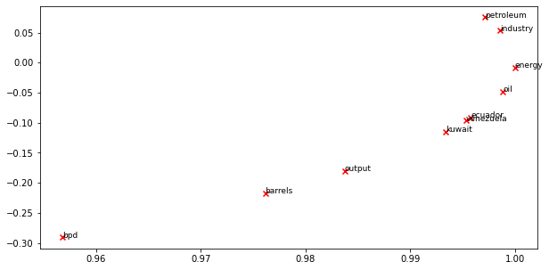
reuters_corpus = read_corpus() M_co_occurrence, word2Ind_co_occurrence = compute_co_occurrence_matrix(reuters_corpus) M_reduced_co_occurrence = reduce_to_k_dim(M_co_occurrence, k=2)
Rescale (normalize) the rows to make them each of unit-length
M_lengths = np.linalg.norm(M_reduced_co_occurrence, axis=1) M_normalized = M_reduced_co_occurrence / M_lengths[:, np.newaxis] # broadcasting
words = [‘barrels’, ‘bpd’, ‘ecuador’, ‘energy’, ‘industry’, ‘kuwait’, ‘oil’, ‘output’, ‘petroleum’, ‘venezuela’] plot_embeddings(M_normalized, word2Ind_co_occurrence, words)
<a name="OWNn2"></a># 基于预测的词向量——word2vec- 加载 word2vec 词向量```pythondef load_word2vec():""" Load Word2Vec VectorsReturn:wv_from_bin: All 3 million embeddings, each lengh 300"""import gensim.downloader as apiwv_from_bin = api.load("word2vec-google-news-300")vocab = list(wv_from_bin.vocab.keys())print("Loaded vocab size %i" % len(vocab))return wv_from_bin
# -----------------------------------# Run Cell to Load Word Vectors# Note: This may take several minutes# -----------------------------------wv_from_bin = load_word2vec()
将 3w word2vec 词向量装入矩阵 M,并使用 TruncatedSVD 降维
def get_matrix_of_vectors(wv_from_bin, required_words=['barrels', 'bpd', 'ecuador', 'energy', 'industry', 'kuwait', 'oil', 'output', 'petroleum', 'venezuela']):""" Put the word2vec vectors into a matrix M.Param:wv_from_bin: KeyedVectors object; the 3 million word2vec vectors loaded from fileReturn:M: numpy matrix shape (num words, 300) containing the vectorsword2Ind: dictionary mapping each word to its row number in M"""import randomwords = list(wv_from_bin.vocab.keys())print("Shuffling words ...")random.shuffle(words)words = words[:10000]print("Putting %i words into word2Ind and matrix M..." % len(words))word2Ind = {}M = []curInd = 0for w in words:try:M.append(wv_from_bin.word_vec(w))word2Ind[w] = curIndcurInd += 1except KeyError:continuefor w in required_words:try:M.append(wv_from_bin.word_vec(w))word2Ind[w] = curIndcurInd += 1except KeyError:continueM = np.stack(M)print("Done.")return M, word2Ind
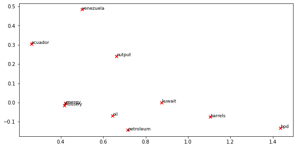
# -----------------------------------------------------------------# Run Cell to Reduce 300-Dimensinal Word Embeddings to k Dimensions# Note: This may take several minutes# -----------------------------------------------------------------M, word2Ind = get_matrix_of_vectors(wv_from_bin) # 将word2vec词向量装入矩阵M_reduced = reduce_to_k_dim(M, k=2) # 降维
绘图
words = ['barrels', 'bpd', 'ecuador', 'energy', 'industry', 'kuwait', 'oil', 'output', 'petroleum', 'venezuela']plot_embeddings(M_reduced, word2Ind, words)
探索多义词 ```python
—————————
Write your polysemous word exploration code here.
wv_from_bin.most_similar(“party”)
—————————
以上代码输出了和“party”最相似的十个单词,可以看出 party 是个多义词,有“派对”的意思,也有“政党”的意思
[(‘Party’, 0.7125184535980225), (‘parties’, 0.6745480298995972), (‘partys’, 0.5965836644172668), (‘Democratic_Party’, 0.5447009801864624), (‘LOUDON_NH_Brad_Keselowski’, 0.5346890687942505), (‘caucus’, 0.522636890411377), (‘pary’, 0.5175394415855408), (‘faction’, 0.5168994665145874), (‘mad_hatter_tea’, 0.507461428642273), (‘Labour_Party’, 0.4938312768936157)]
- 有时候,同义词之间的余弦相似度要低于反义词之间的余弦相似度```python# ------------------# Write your synonym & antonym exploration code here.w1 = "happy"w2 = "cheerful"w3 = "sad"w1_w2_dist = wv_from_bin.distance(w1, w2)w1_w3_dist = wv_from_bin.distance(w1, w3)print("Synonyms {}, {} have cosine distance: {}".format(w1, w2, w1_w2_dist))print("Antonyms {}, {} have cosine distance: {}".format(w1, w3, w1_w3_dist))# ------------------
从以下输出可以看出,虽然“happy”和“cheerful”是同义词,“happy”和“sad”是反义词,但前者之间的余弦距离要大于后者之间的余弦距离:
Synonyms happy, cheerful have cosine distance: 0.6162261962890625Antonyms happy, sad have cosine distance: 0.46453857421875
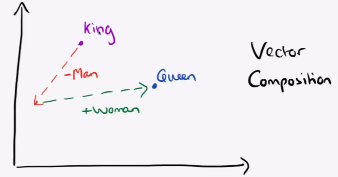
使用词向量实现类比:
# Run this cell to answer the analogy -- man : king :: woman : xpprint.pprint(wv_from_bin.most_similar(positive=['woman', 'king'], negative=['man']))
king + woman - man = queen:
[('queen', 0.7118192911148071),('monarch', 0.6189674139022827),('princess', 0.5902431607246399),('crown_prince', 0.5499460697174072),('prince', 0.5377321243286133),('kings', 0.5236844420433044),('Queen_Consort', 0.5235945582389832),('queens', 0.5181134343147278),('sultan', 0.5098593235015869),('monarchy', 0.5087411999702454)]
但也可能出现错误的类比情况: ```python
—————————
Write your incorrect analogy exploration code here.
pprint.pprint(wv_from_bin.most_similar(positive=[‘china’, ‘japanese’], negative=[‘japan’]))
—————————
输出的并不是 chinese:
[(‘porcelain’, 0.5757269263267517), (‘dinnerware’, 0.563517689704895), (‘crockery’, 0.5430431365966797), (‘silver_flatware’, 0.540193498134613), (‘crystal_stemware’, 0.5391061902046204), (‘flatware’, 0.5293956398963928), (‘tableware’, 0.5281988978385925), (‘china_plates’, 0.5269104838371277), (‘bone_china’, 0.5260535478591919), (‘transferware’, 0.5206524133682251)]
- 词向量中偏见(eg.性别、人种、性取向)的引导分析```python# Run this cell# Here `positive` indicates the list of words to be similar to and `negative` indicates the list of words to be# most dissimilar from.pprint.pprint(wv_from_bin.most_similar(positive=['woman', 'boss'], negative=['man']))print()pprint.pprint(wv_from_bin.most_similar(positive=['man', 'boss'], negative=['woman']))
输出:
[('bosses', 0.5522644519805908),('manageress', 0.49151360988616943),('exec', 0.45940813422203064),('Manageress', 0.45598435401916504),('receptionist', 0.4474116563796997),('Jane_Danson', 0.44480544328689575),('Fiz_Jennie_McAlpine', 0.44275766611099243),('Coronation_Street_actress', 0.44275566935539246),('supremo', 0.4409853219985962),('coworker', 0.43986251950263977)][('supremo', 0.6097398400306702),('MOTHERWELL_boss', 0.5489562153816223),('CARETAKER_boss', 0.5375303626060486),('Bully_Wee_boss', 0.5333974361419678),('YEOVIL_Town_boss', 0.5321705341339111),('head_honcho', 0.5281980037689209),('manager_Stan_Ternent', 0.525971531867981),('Viv_Busby', 0.5256162881851196),('striker_Gabby_Agbonlahor', 0.5250812768936157),('BARNSLEY_boss', 0.5238943099975586)]

若有收获,就点个赞吧
0 人点赞
