Chapter 1 绪论
基本概念术语
- 数据集、样本、属性、属性值、样本空间、特征向量
- 训练、假设、真相(ground-truth)
- 分类、回归、聚类
- 监督学习(分类和回归)、无监督学习(聚类)
- 泛化能力、独立同分布(iid)
-
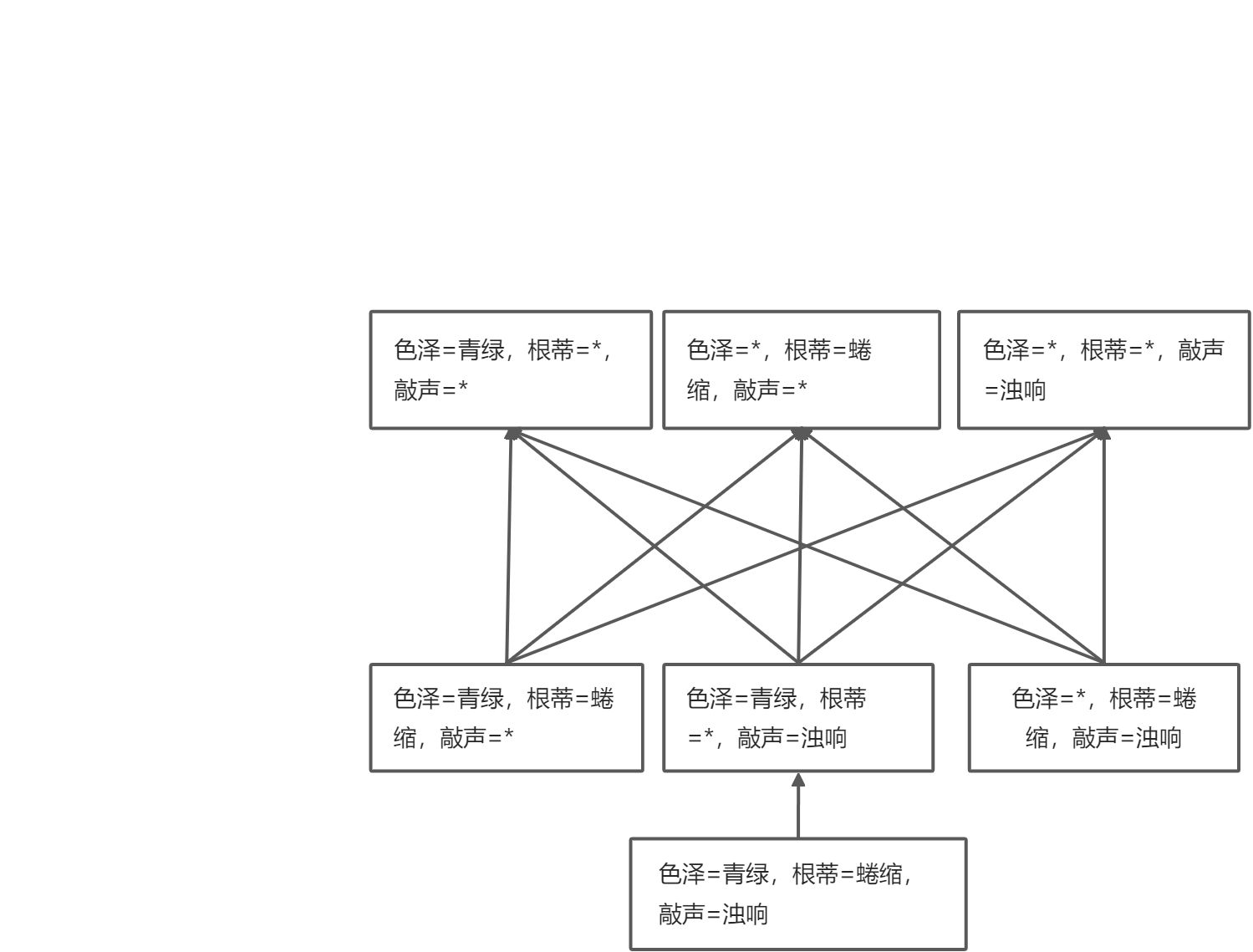
假设空间
空间规模计算
版本空间
一个与训练集一致的“假设集合”


 , 其中
, 其中 为样本总数,
 为分类错误的样本数;
评估方法
留出法(hold-out)
单次使用留出法简洁实现
from sklearn.datasets import load_irisfrom sklearn.model_selection import train_test_split# 加载数据集iris=load_iris()# 得到特征和labelX, y = iris.data, iris.target# 随机将训练集和测试集按照4:1划分X_train, X_test, y_train, y_test = train_test_split(X, y, test_size = 0.2,random_state = 42)
单次使用留出法实现
import numpy as npdef leave_out(X, y, test_size):# 获得所有数据的索引data_index = [idx for idx in range(len(X))]# 打乱索引顺序np.random.shuffle(data_index)# 确定训练和验证的分界线split_index = int((1 - test_size) * len(X))# 训练数据集和验证数据集索引train_data_index = data_index[: split_index]test_data_index = data_index[split_index :]X_train1, X_test1, y_train1, y_test1 = X[train_data_index], X[test_data_index], y[train_data_index], y[test_data_index]return X_train1, X_test1, y_train1, y_test1
交叉验证法(cross validation)
10折交叉验证示意图

- 留一法(
 )
)
优点:不受随机样本的影响,实际评估的模型和期望评估的用完整数据集训练出的模型相似,评估结比较准确
缺点:数据集太大时,计算开销过大
10折交叉验证简洁实现
from sklearn.model_selection import KFoldkf = KFold(n_splits = 10, shuffle = True, random_state = 42)for train_index, test_index, in kf.split(X, y):print('The shape of train_index %s, the shape of test_index %s'%(train_index.shape, test_index.shape))
10折交叉验证实现 ```python import numpy as np def k_fold_split(X, y, n_splits, shuffle=True): n_splits = int(n_splits)
生成索引数组
data_index = np.arange(len(X))
打乱顺序
if shuffle == True:
np.random.shuffle(data_index)
计算每个fold的大小
fold_sizes = np.full(n_splits, len(X) // n_splits) fold_sizes[: len(X) % n_splits] += 1 current = 0 for fold_size in fold_sizes:
# test fold对应的索引位置test_start, test_end = current, current + fold_sizetrain_index = data_index[test_end :]if test_start != 0:train_index = np.concatenate((data_index[: test_start], train_index))test_index = data_index[test_start : test_end]yield (train_index, test_index)current = test_end
for train_index1, test_index1 in k_fold_split(X, y, 14): print(‘The shape of train_index1 %s, the shape of test_index1 %s’ %(train_index1.shape, test_index1.shape))
<a name="EhDcF"></a>### 自助法(bootstrapping)- 示意图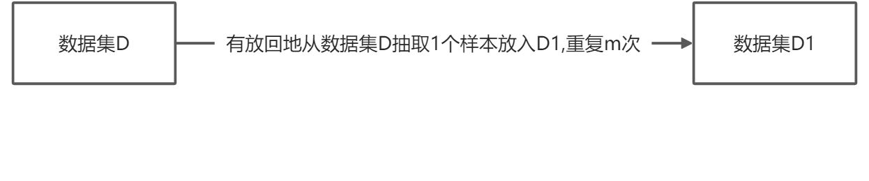- 当样本数目足够多时,次抽样始终不被抽到的概率趋近于- 自助法使用pandas实现```pythonimport pandas as pddf_X = pd.DataFrame(X, columns=['SepalLengthCm', 'SepalWidthCm', 'PetalLengthCm', 'PetalWidthCm'])df_y = pd.DataFrame(y, columns=['Species'])# 将X和y的Dataframe在列上相连df = pd.concat([df_X, df_y], axis = 1)# 采样train = df.sample(frac = 1.0, replace = True)# 没有采样到的作为testtest = df.loc[df.index.difference(train.index)].copy()# 转成ndarrayX_train2, y_train2 = train.iloc[:,[0, 1, 2, 3]].values, train.iloc[:, 4].valuesX_test2, y_test2 = test.iloc[:, [0, 1, 2, 3]].values, test.iloc[:, 4].valuesX_train2.shape, X_test2.shape
自助法实现
import numpy as nptrain_index = np.random.randint(len(X), size=len(X))bool_index = np.zeros(len(X), dtype = bool)bool_index[train_index] = Truetest_index = np.argwhere(bool_index == False).reshape(-1)X_train3, y_train3, X_test3, y_test3 = X[train_index], y[train_index], X[test_index], y[test_index]X_train3.shape, X_test3.shape
性能度量
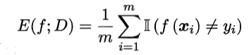
错误率和精度
错误率公式
- 精度公式

精度简洁实现
import numpy as npy_pred = np.random.randint(0, 3, size = y.shape)from sklearn.metrics import accuracy_scoreprint(accuracy_score(y, y_pred))
精度实现
acc_cnt = 0for i in range(len(y)):if y[i] == y_pred[i]:acc_cnt += 1print(acc_cnt / len(y))
查准率、查全率和F1
二分类问题的混淆矩阵

tips: TP的P表示预测为positive,T表示预测对了:true。 同理,TN表示预测为Negative,并且预测对了:true
- 查准率
 和查全率
和查全率


- 多分类问题的
 和
和
“宏查全率”、“宏查准率”、“宏F1”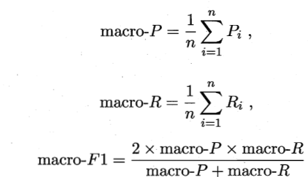
“微查全率”、“微查准率”、“微F1”


宏和微指标的区别是宏是先算指标再平均,微是先把TP,FP,TN以及FN平均,再算指标
查准率和查全率简洁实现
from sklearn.metrics import precision_score, recall_score, f1_scoreprint('宏查准率:', precision_score(y, y_pred, average = 'macro'))print('宏查全率:', recall_score(y, y_pred, average = 'macro'))print('宏F1 Score:', f1_score(y, y_pred, average = 'macro'))
查准率和查全率实现(三分类) ```python def get_score(y, y_pred, label): TP, TN, FP, FN = 0, 0, 0, 0 for i in range(len(y)):
if y[i] == label and y_pred[i] == label:TP += 1elif y[i] == label and y_pred[i] != label:FN += 1elif y[i] != label and y_pred[i] == label:FP += 1elif y[i] != label and y_pred[i] != label:TN += 1
return [TP, TN, FP, FN]
score_0 = get_score(y, y_pred, 0) p_0 = score_0[0] / (score_0[0] + score_0[2]) r_0 = score_0[0] / (score_0[0] + score_0[3]) f1_0 = 2 p_0 r_0 / (p_0 + r_0) score_1 = get_score(y, y_pred, 1) p_1 = score_1[0] / (score_1[0] + score_1[2]) r_1 = score_1[0] / (score_1[0] + score_1[3]) f1_1 = 2 p_1 r_1 / (p_1 + r_1) score_2 = get_score(y, y_pred, 2) p_2 = score_2[0] / (score_2[0] + score_2[2]) r_2 = score_2[0] / (score_2[0] + score_2[3]) f1_2 = 2 p_2 r_2 / (p_2 + r_2) macro_p = (p_0 + p_1 + p_2) / 3 macro_r = (r_0 + r_1 + r_2) / 3 macro_f1 = 2 macro_p macro_r / (macro_p + macro_r) macro_f1_1 = (f1_0 + f1_1 + f1_2) / 3 print(‘macro precision score:’, macro_p) print(‘macro recall score:’, macro_r) print(‘macro f1 score:’, macro_f1) print(‘macro f1 score:’, macro_f1_1) ``` notes:计算macro-F1,micro-F1有两种方式,一种是西瓜书提到的公式,另一种是把对所有F1作平均。具体两种方法的差别可以看 https://arxiv.org/pdf/1911.03347.pdf,比较推荐求出所有F1,再作平均的方法(sklearn使用的这种)

若有收获,就点个赞吧
0 人点赞
