gghalves：画半图，sao气逼人

• 该包让half-half图的实现变得更容易，比如一张图，左边一半是散点右边一半是小提琴
• 特点：基于ggplot2的语法，用以下函数，来拓展选定的geom
  • geom_half_boxplot
  • geom_half_violin
  • geom_half_point ```

    安装该包

    if (!require(devtools)) { install.packages(‘devtools’) } devtools::install_github(‘erocoar/gghalves’)

加载包，用iris数据感受一下

library(ggplot2) library(gghalves)

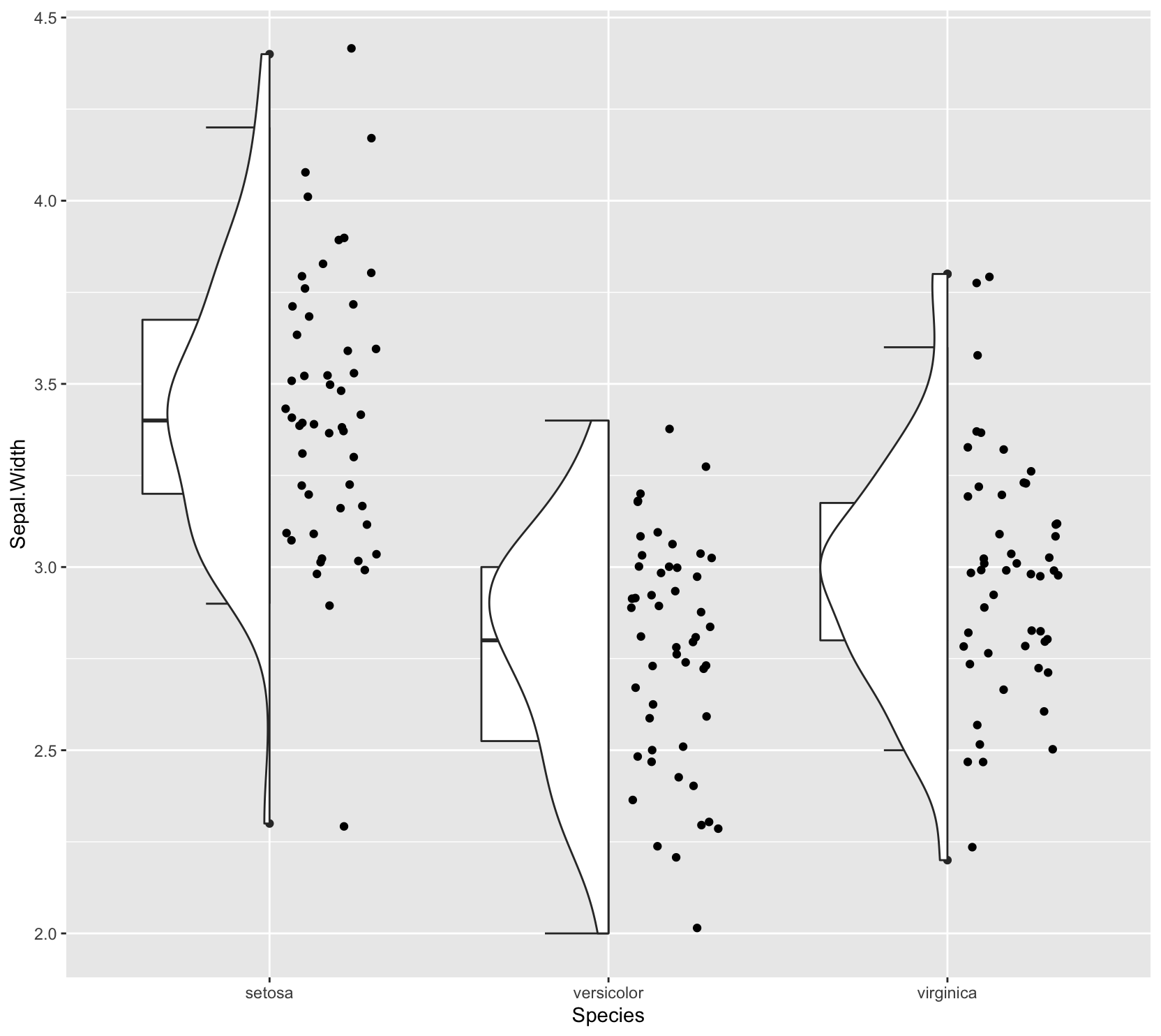
基础版

ggplot(iris, aes(x = Species, y = Sepal.Width)) + geom_half_point() + geom_half_boxplot() + geom_half_violin()

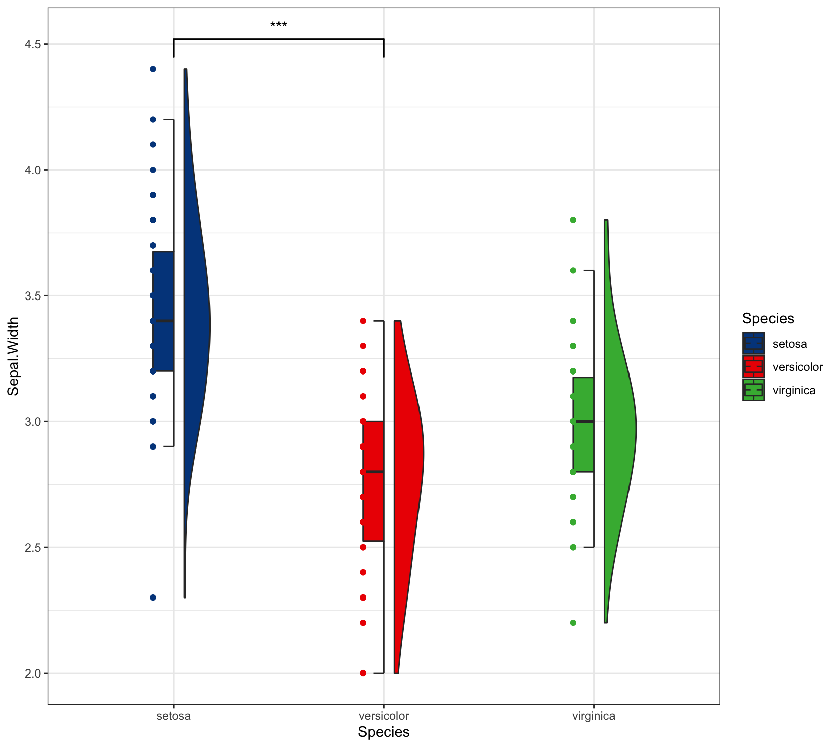
进阶版

library(ggplot2) library(gghalves) library(ggsci) library(ggpubr)

ggplot(iris, aes(x = Species, y = Sepal.Width, fill = Species) ) + geom_half_violin( aes(fill = Species), adjust = 1.5, position = position_nudge(x = 0.05), width = 0.3, side = “r”) + geom_half_boxplot(aes(fill = Species), outlier.shape = NA, width = 0.2) + geom_point(aes(x = as.numeric(Species) -0.1, #注意先画前面两个半图，最后画geom_point y = Sepal.Width, colour = Species)) + scale_fill_lancet() + scale_color_lancet() + geom_signif(comparisons = list(c(“setosa”, “versicolor”)), map_signif_level = c(“*” = 0.001, ““ = 0.01, “*” = 0.5)) + theme_bw()

![plot_zoom_png.png](https://cdn.nlark.com/yuque/0/2021/png/21884283/1638810428978-272e143b-a798-4b8a-926a-8b93223b90e3.png#clientId=u5c8f9629-7a33-4&crop=0&crop=0&crop=1&crop=1&from=drop&height=353&id=uffa5913c&margin=%5Bobject%20Object%5D&name=plot_zoom_png.png&originHeight=1484&originWidth=1664&originalType=binary&ratio=1&rotation=0&showTitle=false&size=156226&status=done&style=none&taskId=u99babea6-a983-4d2b-a04c-883eac31969&title=&width=396)![plot_zoom_png.png](https://cdn.nlark.com/yuque/0/2021/png/21884283/1638812373300-23bdfee1-b468-4ce2-b7ee-1953c923f8ed.png#clientId=u5c8f9629-7a33-4&crop=0&crop=0&crop=1&crop=1&from=drop&height=381&id=u4353536a&margin=%5Bobject%20Object%5D&name=plot_zoom_png.png&originHeight=1484&originWidth=1664&originalType=binary&ratio=1&rotation=0&showTitle=false&size=129448&status=done&style=none&taskId=u792af89c-331a-4eb0-8301-24424b67f37&title=&width=427)
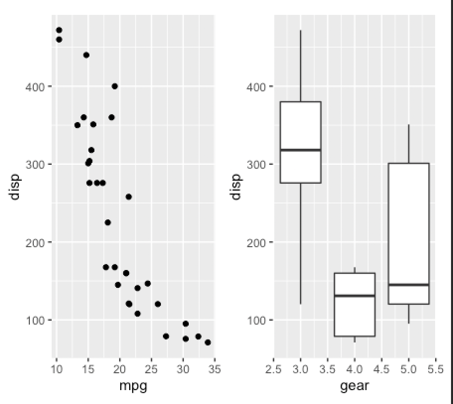
- 可选参数：
   - side：= l 把半图放左边，= r 把半图放右边
**patchwork包: 灰常灰常强大的拼图，大家一定要一起学，值得入手！！**<br />这个包学习的时候，可以把待拼图的画布想象成一个网格grid，你想在哪一块画图，就往里面填
- 特点：+即可拼图
- 由于该包是针对于ggplot2，所以对ggplo2或者ggplot2的延展包可以很好的适用。但对其他非ggplot2的包的图就不适用了，如pheatmap的热图，可以使用AI或者其他拼图软件完成。

library(patchwork)

p1 <- ggplot(mtcars) + geom_point(aes(mpg, disp)) p2 <- ggplot(mtcars) + geom_boxplot(aes(gear, disp, group = gear)) p1 + p2

![Screen Shot 2021-12-06 at 9.42.46 PM.png](https://cdn.nlark.com/yuque/0/2021/png/21884283/1638823377224-f2dcffbd-1a6b-42f6-b697-3d039667b294.png#clientId=ub0651bbd-9639-4&crop=0&crop=0&crop=1&crop=1&from=drop&height=427&id=ua1a313a1&margin=%5Bobject%20Object%5D&name=Screen%20Shot%202021-12-06%20at%209.42.46%20PM.png&originHeight=814&originWidth=912&originalType=binary&ratio=1&rotation=0&showTitle=false&size=448192&status=done&style=none&taskId=u43c4b691-24cb-484a-9fa0-88f9b31573f&title=&width=478)

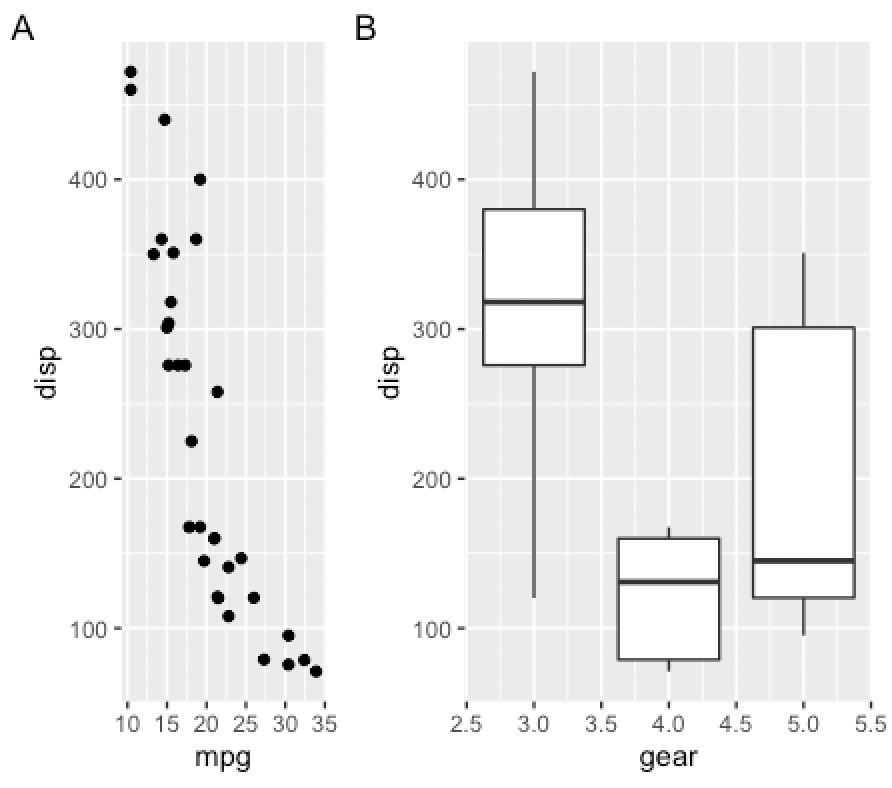
plot_layout:可以对图形排列以及每个图的范围进行指定

p1 + p2 +plot_layout(ncol = 1, heights = c(4,1)) p1 + p2 + plot_layout(ncol = 2, width = c(1, 2)) + plot_annotation(tag_levels = ‘A’) #添加标记

plot_spacer()填充空白格

p1 + plot_spacer() + p2

![Screen Shot 2021-12-06 at 9.43.17 PM.png](https://cdn.nlark.com/yuque/0/2021/png/21884283/1638823409166-bf43fc6e-2f61-469f-b490-a4392db8001b.png#clientId=ub0651bbd-9639-4&crop=0&crop=0&crop=1&crop=1&from=drop&height=460&id=u2ee734cb&margin=%5Bobject%20Object%5D&name=Screen%20Shot%202021-12-06%20at%209.43.17%20PM.png&originHeight=788&originWidth=892&originalType=binary&ratio=1&rotation=0&showTitle=false&size=471116&status=done&style=none&taskId=uf46ea16e-497b-417d-9ea8-32360c3983b&title=&width=521)

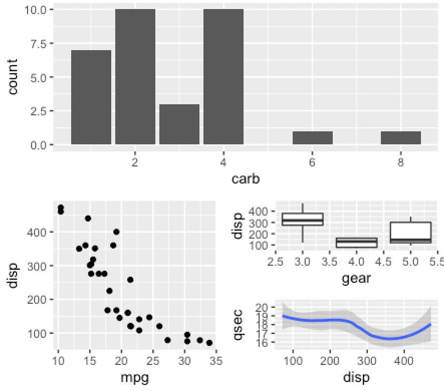
增加花括号的使用进行嵌套可以布置更复杂的图形：

p3 <- ggplot(mtcars) + geom_smooth(aes(disp, qsec)) p4 <- ggplot(mtcars) + geom_bar(aes(carb)) p4 + { p1 + { p2 + p3 + plot_layout(ncol = 1) } } + plot_layout(ncol = 1)

![Screen Shot 2021-12-06 at 9.44.21 PM.png](https://cdn.nlark.com/yuque/0/2021/png/21884283/1638823472802-297cfde9-6f49-4450-a885-8bd81e63320a.png#clientId=ub0651bbd-9639-4&crop=0&crop=0&crop=1&crop=1&from=drop&height=403&id=u2fe50e28&margin=%5Bobject%20Object%5D&name=Screen%20Shot%202021-12-06%20at%209.44.21%20PM.png&originHeight=780&originWidth=886&originalType=binary&ratio=1&rotation=0&showTitle=false&size=364307&status=done&style=none&taskId=u8b7a6139-4db4-4803-a527-f8e8779a859&title=&width=458)

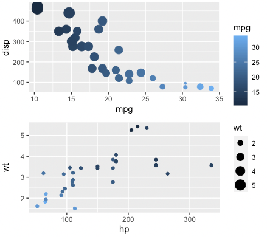
plot_layout()

p5 <- ggplot(mtcars) + geom_point(aes(mpg, disp, colour = mpg, size = wt)) p6 <- ggplot(mtcars) + geom_point(aes(hp, wt, colour = mpg)) 3 p5 + p6 + plot_layout(guides = ‘collect’) #收集图例，去除重复图例

![Screen Shot 2021-12-06 at 9.45.11 PM.png](https://cdn.nlark.com/yuque/0/2021/png/21884283/1638823523347-9349a589-640b-4b6b-8a6b-4f5ec052e913.png#clientId=ub0651bbd-9639-4&crop=0&crop=0&crop=1&crop=1&from=drop&height=389&id=u7f153bf8&margin=%5Bobject%20Object%5D&name=Screen%20Shot%202021-12-06%20at%209.45.11%20PM.png&originHeight=780&originWidth=878&originalType=binary&ratio=1&rotation=0&showTitle=false&size=338292&status=done&style=none&taskId=ua379a5cc-377d-4419-8967-0cb5dd6a232&title=&width=438)<br />**design: 自由设计图形格式，非常灵活便捷**

p1 <- ggplot(mtcars) + geom_point(aes(mpg, disp)) p2 <- ggplot(mtcars) + geom_boxplot(aes(gear, disp, group = gear)) p3 <- ggplot(mtcars) + geom_bar(aes(gear)) + facet_wrap(~cyl) p4 <- ggplot(mtcars) + geom_bar(aes(carb)) p5 <- ggplot(mtcars) + geom_violin(aes(cyl, mpg, group = cyl))

design: 自由设计图形格式，非常灵活便捷， ##note：”#”代表一个空格，每个字母代表占用一个格子

design <- “

BB

AACD AA#D
“

p1 + p2 + p3 + p4 + p5 + plot_layout(design = design) ```