- pycharm的console/cmd
- 技巧
- bug
- 语法基础
- 数据结构
- 类与继承
- 创建父类
class person:
#若加上:slots=(‘fname’,’lname’) 则表明init里只能创建fname和lname这两个参数,如果再加上其他的参数则运行错误
def init(self, fname, lname):
self.firstname = fname
self.lastname = lname
def printname(self):
print(self.firstname , self.lastname)
#子类
class student(person): #表示继承父类
def init(self,fname,lname,year): #若不写super(),则子类的init会覆盖父类的init
super().init(fname,lname)
self.graduationyear = year #添加year参数
x=student(“elon”,’musk’,2016)
print(x.graduationyear)
#2016 - numpy
- pandas
- a是数据,如np.random.randn(8, 4),c是列名
- matplotlib
- 数据清洗
- 爬虫
- camelot:提取pdf里的表格
- 用百度ai提取图片表格并转换为excel(推荐)
- https://aip.baidubce.com/oauth/2.0/token?grant_type=client_credentials&client_id=hTsFtKOkCgolR2eG1d68AHUT&client_secret=1W2EI6YhMeAYuk7eh0u1Z6ghBvXDNETE‘
response = requests.get(host)
if response:
print(response.json())
# ‘access_token’: ‘24.3282cb4d662b947c6e1d1e501f69fc31.2592000.1596958041.282335-21237240’
#step2:提交请求接口,获取request_id
request_url = “https://aip.baidubce.com/rest/2.0/solution/v1/form_ocr/request“
# 二进制方式打开图片文件
f = open(‘tabletest1.jpg’, ‘rb’)
img = base64.b64encode(f.read())
params = {“image”: img}
access_token = ‘24.3282cb4d662b947c6e1d1e501f69fc31.2592000.1596958041.282335-21237240’
request_url = request_url + “?access_token=” + access_token
headers = {‘content-type’: ‘application/x-www-form-urlencoded’}
response = requests.post(request_url, data=params, headers=headers)
# 若:response = requests.post(request_url, data=params, headers=headers,is_sync=True) 则同步返回同步返回识别结果,无需调用获取结果接口。
if response:
print (response.json())
# step3:获取结果
request_url = ‘https://aip.baidubce.com/rest/2.0/solution/v1/form_ocr/get_request_result‘
params = {‘request_id’: ‘21237240_1953321’} # 每执行一次“提交请求接口”,request_id都会变
access_token = ‘24.3282cb4d662b947c6e1d1e501f69fc31.2592000.1596958041.282335-21237240’
request_url = request_url + “?access_token=” + access_token
headers={‘Content-Type’:’application/x-www-form-urlencoded’}
response = requests.post(request_url, data=params, headers=headers)
if response:
print (response.json())">需要每次更换的是:request_id和access_token;
#client_id/secret的有效期是一个月左右
# encoding:utf-8
import requests
import base64
# step1:获取access_token
# client_id 为官网获取的AK, client_secret 为官网获取的SK
host = ‘https://aip.baidubce.com/oauth/2.0/token?grant_type=client_credentials&client_id=hTsFtKOkCgolR2eG1d68AHUT&client_secret=1W2EI6YhMeAYuk7eh0u1Z6ghBvXDNETE‘
response = requests.get(host)
if response:
print(response.json())
# ‘access_token’: ‘24.3282cb4d662b947c6e1d1e501f69fc31.2592000.1596958041.282335-21237240’
#step2:提交请求接口,获取request_id
request_url = “https://aip.baidubce.com/rest/2.0/solution/v1/form_ocr/request“
# 二进制方式打开图片文件
f = open(‘tabletest1.jpg’, ‘rb’)
img = base64.b64encode(f.read())
params = {“image”: img}
access_token = ‘24.3282cb4d662b947c6e1d1e501f69fc31.2592000.1596958041.282335-21237240’
request_url = request_url + “?access_token=” + access_token
headers = {‘content-type’: ‘application/x-www-form-urlencoded’}
response = requests.post(request_url, data=params, headers=headers)
# 若:response = requests.post(request_url, data=params, headers=headers,is_sync=True) 则同步返回同步返回识别结果,无需调用获取结果接口。
if response:
print (response.json())
# step3:获取结果
request_url = ‘https://aip.baidubce.com/rest/2.0/solution/v1/form_ocr/get_request_result‘
params = {‘request_id’: ‘21237240_1953321’} # 每执行一次“提交请求接口”,request_id都会变
access_token = ‘24.3282cb4d662b947c6e1d1e501f69fc31.2592000.1596958041.282335-21237240’
request_url = request_url + “?access_token=” + access_token
headers={‘Content-Type’:’application/x-www-form-urlencoded’}
response = requests.post(request_url, data=params, headers=headers)
if response:
print (response.json()) - 多层神经网络
pycharm的console/cmd
- 清除一个变量:del 变量名
- 清楚所有变量:先输入reset ,回车后再输入y
- 在cmd里查看包的位置,输入pip show 包名
- 在cmd里删除包,pip uninstall 包名
技巧
#显示所有列pd.set_option('display.max_columns', None)#显示所有行pd.set_option('display.max_rows', None)#dataframe的日期只提取年月dataframe.dt.strftime('%Y-%m')
bug
- no model found
解决办法:
import syssys.path.append(r'上一级的绝对路径')
语法基础
print(f’’):格式化输出,‘’里变量用方括号括起
在console中用”def 变量名”来删除变量
- 在变量前后使用“?”,可以显示对象信息
In [10]: print?
Docstring:
print(value, …, sep=’ ‘, end=’\n’, file=sys.stdout, flush=False)
- 强行终止:代码运行时按Ctrl-C,无论是%run或长时间运行命令,都会导致
KeyboardInterrupt。这会导致几乎所有Python程序立即停止,除非一些特殊情况。 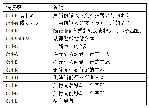

- Python的语句不需要用分号结尾。但是,分号却可以用来给同在一行的语句切分
错误处理
try:# 语句except Exception as e:print(e)else:# 语句
输入输出
输入:x = input([‘输入提示’])
# 输入获得两个字符串(如输入abd def或abc,def)x,y=input('Input: ').split()x,y=input('Input: ').split(',')# 输入获得两个整数x,y = eval(input('Input: '))# 输入后获得一个元素均为数值型的列表lst = list(eval(input('Input: '))) #输入12,3.4,456lst = eval(input('Input: ')) # 输入[12,3.4,456]
输出:print(object1,obk=ject2,…,sep = ‘’, end = ‘\n’)
sep表示输出对象之间的分隔符,默认为空格;参数end的默认值为’\n’,表示print()函数输出完成后自动换行
# 在输出数据中加入一个空白分隔符print(x,y,sep = ',') # 用逗号分隔print(x),print(y) # 换行#循环输出所有的数据并放在同一行输出for i in range(1,5):print(i, end=' ')#格式化输出print(format.)print(format_string.format(arguments_to_convert))
for循环
1、用for遍历字典
a={'':,'':}for i in a.keys():#操作for i in a.values():#操作#同时提出键和值a.items()
数据结构
| 顺序 | 能否更改 | 能否重复 | 表达 | 有无索引 | 其他 | |
|---|---|---|---|---|---|---|
| 列表 list |
能 | 1)[…]; 2)创建方法:list(range()); a=[i**2 for i in range(0,5)] |
1、排序。从小到大:a.sort();从大到小:a.sort(reverse=True) 2、一个列表可以放任何类型的数据;列表里面可以包含列表 |
|||
| 元组 | 有序 | 不能 | 能 | ( , , , ) e.g:In: tuple([4, 0, 2]) Out: (4, 0, 2) |
可以用方括号”[ ]”访问元组中的元素 | 1、用tuple可以将任意序列或迭代器转换成元组2、可以用加号运算符将元组串联起来 In: (4, None, ‘foo’) + (6, 0) Out: (4, None, ‘foo’, 6, 0) 3、简便的替换 a,b=b,a |
| 集合 | 无序 | 不能 | 不能 | 可以把它当做字典,但是只有键没有值 | ||
| 字符串 | 1、字符串只能和字符串相加,str() |
- range(start, end, step),返回一个list对象也就是range.object,起始值为start,终止值为end,但不含终止值,步长为step。只能创建int型list。
- arange(start, end, step),与range()类似,也不含终止值。但是返回一个array对象。需要导入numpy模块(import numpy as np或者from numpy import*),并且arange可以使用float型数据。
- 切片:左闭右开
- 查看元素类型:type(变量名)
- range(起始,终止,步长),但终止值不包含,用list可转化为列表
python的所有编号都是从0开始的
seq = [7, 2, 3, 7, 5, 6, 0, 1]# 隔取In [81]: seq[::2]Out[81]: [7, 3, 3, 6, 1]# 逆序In [82]: seq[::-1]Out[82]: [1, 0, 6, 5, 3, 6, 3, 2, 7]
类与继承
创建父类
class person:
#若加上:slots=(‘fname’,’lname’) 则表明init里只能创建fname和lname这两个参数,如果再加上其他的参数则运行错误
def init(self, fname, lname):
self.firstname = fname
self.lastname = lname
def printname(self):
print(self.firstname , self.lastname)
#子类
class student(person): #表示继承父类
def init(self,fname,lname,year): #若不写super(),则子类的init会覆盖父类的init
super().init(fname,lname)
self.graduationyear = year #添加year参数
x=student(“elon”,’musk’,2016)
print(x.graduationyear)
#2016numpy
创建数组:np.array([···]);表示先创建一个列表[],然后把用np.array列表转化为np里的数组
- python里的矩阵用np里的二维数组表示
- np.concatenate((要合并的矩阵(可以多个)),axis=) #axis=1按行合并;axis=0 按列合并
- 不等量分割: np.array_split
- 关于axis这个属性的定义是基于数组shape的这个属性,它是一个python元组,对于二维书而言,axi
np.array生成数组,用np.dot()表示矩阵乘积;(*)号或np.multiply()表示点乘
np.mat生成数组,(*)和np.dot()相同,点乘只能用np.multiply()
总结下来, dot()一定是点乘,multiply()一定是对应位置的元素相乘。数据切片:https://www.jianshu.com/p/15715d6f4dad
# 从Excel导入文件.但一般用pandas导入import numpy as npa = np.genfromtext(r':\',dytpe=,delimiter=',',skip=)#delimiter表示分隔符号# skip:要不要跳过第一行,为0表示不跳过数据的首行;为1表示从第二行开始输入
pandas
dataframe:行的索引是index,列的索引是columns,数据是numpy的数据 ```python df=pd.DataFrame(a ,index=b, columns=c)
a是数据,如np.random.randn(8, 4),c是列名
df[[‘column1’,’culumn2’,…]] #选出列 df[:2] #选出前两行
df.loc[:,’’] #[]左边为index,右边为column。 loc有点像excel的鼠标左键,可以随意拉动需要的数据
1、pd.DataFrame(数据,index=.columns=)<br />也可以用字典,字典的索引是列标<br />将dataframe导出为excel : xxx.to_excel('XX.xls')<br />#select by index<br />.col 以标签的形式选择<br />#select by position: iloc<br />#mixed selection: ix<br /># 0是对行处理(以行为对象),1是对列处理<br />#isnull()看是否缺失<br />#fillna()- py普通的切片不包括尾部数值,但Series不同<a name="cnPLD"></a>## 数据分析<a name="HjjS1"></a>### 数据探索与清洗```pythonimport pandas as pddata = pd.read_csv(".txt",sep='',names=[])'''1\关联两个表数据 =pd.merge(data1,data2)2\提取所需要的列 =pd.DataFrame(data,columns=[])3\查看前num行数据 data.head(num)''''''假设数据集为data'''# 首先查看数据信息data.shape # 查看数据规模——多少行,多少列data.info() # 查看整体数据信息,包括每个字段的名称、非空数量、字段的数据类型data.describe() # 查看数据分布#数据清理data['ColName'].filna('ReplaceName',inplace='') # 空值处理data['ColName']=data['ColName'].astype(datatype) # 转换数据类型如str,float
数据分析
data.groupby('ColName').sum().sort_values('ColName2',ascending=True/False).head(num)
matplotlib
import matplotlib.pyplot as pltimport numpy as np# 有了sharex和sharey会比较好看:不会重合,有空隙'''fig, axs = plt.subplots(2,2,sharex=True,sharey=True) # a figure with a 2x2 grid of Axes :(0,0)x = np.linspace(0,2,100)axs[1,1].plot(x,x,label='linear')axs[1,0].plot(x,x**2,label='quadratic')axs[1,1].set_xlabel('xlabel')axs[1,1].set_ylabel('ylabel')axs[1,1].set_title('Simple Plot')axs[1,1].legend()plt.show()'''# method 2''' fig = plt.figure()ax1 = fig.add_subplot(2,2,1)'''# method 3'''fig, (ax1, ax2) = plt.subplots(1, 2)my_plotter(ax1, data1, data2, {'marker': 'x'})'''data = {'a' : np.arange(50),'b' : np.random.randint(0,50,50),'d': np.random.randn(50)}plt.xlabel('entry a')plt.ylabel('entry b')plt.show()
plt.rcParams[]
pylot使用rc配置文件来自定义图形的各种默认属性,称之为rc配置或rc参数。通过rc参数可以修改默认的属性,包括窗体大小、每英寸的点数、线条宽度、颜色、样式、坐标轴、坐标和网络属性、文本、字体等。
rc参数存储在字典变量中,通过字典的方式进行访问,如下代码:
数据清洗
就是把数据从数值、格式等方面规范化。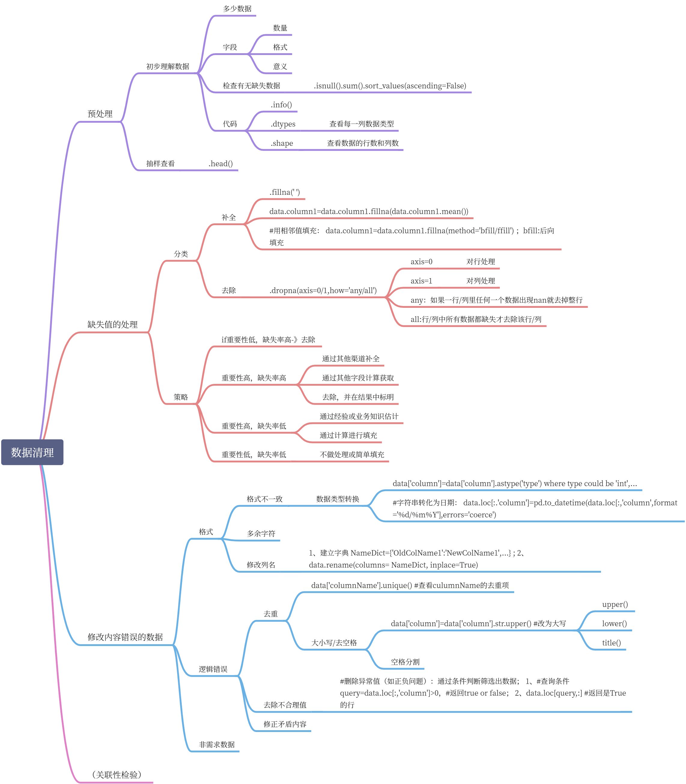
import pandas as pdimport numpy as npori_data = pd.read_excel('E:\\test.xlsx')data = pd.DataFrame(ori_data)data.head()colname = {'Unnamed: 0':'age'}data.rename(columns=colname, inplace=True)# .dropna():只要包含nan的行都删除newdata = data.dropna(axis=1,how='any') # 只有当一列中所有值都是NA时才删除该列newdata.loc['total']=newdata['total'].astype(np.float)pd.set_option('display.max_columns', 1000)pd.set_option('display.width', 1000)pd.set_option('display.max_colwidth', 1000)newdata=newdata.dropna(how='any') # delete the row(s) with nanprint(newdata)
#补全缺失值.fillna()括号里可以是字典({column:value,...})或数字# 删除重复行:.drop_duplicates();制定子集:.drop_duplicates(['column'])
爬虫
网络数据获取
import requests# 当爬取的网站有反爬虫机制时,要向服务器发出爬虫请求,需要添加请求头:headers#把user-agent换成自己电脑的user-agent。查找办法,在浏览器上输入about:version,#用户代理那一行显示的就是自己电脑的user-agentheaders = {'User-Agent':'Mozilla/5.0 (Windows NT 10.0; Win64; x64)\ # \:换行符AppleWebKit/537.36 (KHTML, like Gecko) Chrome/83.0.4103.97 Safari/537.36'}url = 'https://movie.douban.com/subject/33477335/comments/' # 要爬取数据的网址r=requests.get(url,headers=headers)print(r.status_code)#完整程序import requestsfrom bs4 import BeautifulSoupimport re # re正则表达式模块进行各类正则表达式处理headers = {'User-Agent':'Mozilla/5.0 (Windows NT 10.0; Win64; x64) AppleWebKit/537.36 (KHTML, like Gecko) Chrome/83.0.4103.97 Safari/537.36'}url = 'https://movie.douban.com/subject/33477335/comments/'r = requests.get(url, headers=headers)# 用beautifulsoup 传入字符串, 获得beautifulsoup对象soupsoup = BeautifulSoup(r.text,'lxml')pattern = soup.find_all('span','short') #pattern是一个列表for item in pattern:print(item.string)pattern_s = re.compile('<span class="user-stars allstar(.*?) rating"')p = re.findall(pattern_s, r.text)s=0for star in p:s += int(star)print(s)
爬虫核心程序
import requestsimport reheaders={'User-Agent':"Mozilla/5.0 (Windows NT 10.0; Win64; x64) AppleWebKit/537.36 (KHTML, like Gecko) Chrome/83.0.4103.97 Safari/537.36"}def baidu(company):url='https://www.baidu.com/s?rtt=1&bsst=1&cl=2&tn=news&ie=utf-8&word='+companyres = requests.get(url, headers=headers).text# 提取超链接p_href = '<h3 class="news-title_1YtI1"><a href="(.*?)"'href=re.findall(p_href,res,re.S)# 提取题目p_title= '<h3 class="news-title_1YtI1">.*?>(.*?)</a>'title = re.findall(p_title,res,re.S)# 提取日期p_date = '<span class="c-color-gray2 c-font-normal">(.*?)</span>'date = re.findall(p_date,res)p_source = '<span class="c-color-gray c-font-normal c-gap-right">(.*?)</span>'source = re.findall(p_source,res)for i in range(len(title)):title[i]=title[i].strip() # strip()用来取消字符串两端的换行或空格title[i]=re.sub(r'<.*?>','',title[i])title[i] = re.sub(r'\u200b','',title[i])file = open(r'F:\数据挖掘报告.txt','a')file.write(str(company) + '\n')for i in range(len(title)):file.write(str(i+1)+'.'+title[i]+'('+date[i]+'-'+source[i]+')'+'\n')file.write(href[i]+'\n')file.write('--------------------'+'\n')company=['华为','阿里巴巴','美团','饿了吗']for i in company:baidu(i)
camelot:提取pdf里的表格
import camelottables = camelot.read_pdf('E:\\XXX\\文件名.pdf',flavor='stream',pages='6') # 一定要写flavor='stream'tables[0].dftables.export('XXX.xls',f='excel',compress = False)plt = camelot.plot(tables[0],kind='text')plt.show() #查看图表位置
用百度ai提取图片表格并转换为excel(推荐)
需要每次更换的是:request_id和access_token;
#client_id/secret的有效期是一个月左右
# encoding:utf-8
import requests
import base64
# step1:获取access_token
# client_id 为官网获取的AK, client_secret 为官网获取的SK
host = ‘https://aip.baidubce.com/oauth/2.0/token?grant_type=client_credentials&client_id=hTsFtKOkCgolR2eG1d68AHUT&client_secret=1W2EI6YhMeAYuk7eh0u1Z6ghBvXDNETE‘
response = requests.get(host)
if response:
print(response.json())
# ‘access_token’: ‘24.3282cb4d662b947c6e1d1e501f69fc31.2592000.1596958041.282335-21237240’
#step2:提交请求接口,获取request_id
request_url = “https://aip.baidubce.com/rest/2.0/solution/v1/form_ocr/request“
# 二进制方式打开图片文件
f = open(‘tabletest1.jpg’, ‘rb’)
img = base64.b64encode(f.read())
params = {“image”: img}
access_token = ‘24.3282cb4d662b947c6e1d1e501f69fc31.2592000.1596958041.282335-21237240’
request_url = request_url + “?access_token=” + access_token
headers = {‘content-type’: ‘application/x-www-form-urlencoded’}
response = requests.post(request_url, data=params, headers=headers)
# 若:response = requests.post(request_url, data=params, headers=headers,is_sync=True) 则同步返回同步返回识别结果,无需调用获取结果接口。
if response:
print (response.json())
# step3:获取结果
request_url = ‘https://aip.baidubce.com/rest/2.0/solution/v1/form_ocr/get_request_result‘
params = {‘request_id’: ‘21237240_1953321’} # 每执行一次“提交请求接口”,request_id都会变
access_token = ‘24.3282cb4d662b947c6e1d1e501f69fc31.2592000.1596958041.282335-21237240’
request_url = request_url + “?access_token=” + access_token
headers={‘Content-Type’:’application/x-www-form-urlencoded’}
response = requests.post(request_url, data=params, headers=headers)
if response:
print (response.json())
post函数的请求参数
| 参数 | 是否必选 | 类型 | 可选值范围 | 说明 |
|---|---|---|---|---|
| image | 是 | string | - | 图像数据,base64编码后进行urlencode,要求base64编码和urlencode后大小不超过4M,最短边至少15px,最长边最大4096px,支持jpg/jpeg/png/bmp格式 |
| is_sync | 否 | string | true/false | 是否同步返回识别结果。取值为“false”,需通过获取结果接口 获取识别结果;取值为“true”,同步返回识别结果,无需调用获取结果接口。默认取值为“false” |
| request_type | 否 | string | json/excel | 当 is_sync=true 时,需在提交请求时即传入此参数指定获取结果的类型,取值为“excel”时返回xls文件的地址,取值为“json”时返回json格式的字符串。当 is_sync=false 时,需在获取结果时指定此参数。 |
# encoding:utf-8import requestsimport base64# step1:获取access_token# client_id 为官网获取的AK, client_secret 为官网获取的SKhost = 'https://aip.baidubce.com/oauth/2.0/token?grant_type=client_credentials&client_id=hTsFtKOkCgolR2eG1d68AHUT&client_secret=1W2EI6YhMeAYuk7eh0u1Z6ghBvXDNETE'response = requests.get(host)if response:print(response.json())# 提交请求接口# 'access_token': '24.3282cb4d662b947c6e1d1e501f69fc31.2592000.1596958041.282335-21237240'#step2:提交请求接口request_url = "https://aip.baidubce.com/rest/2.0/solution/v1/form_ocr/request"# 二进制方式打开图片文件f = open('tabletest1.jpg', 'rb')img = base64.b64encode(f.read())params = {"image": img}access_token = '24.3282cb4d662b947c6e1d1e501f69fc31.2592000.1596958041.282335-21237240'request_url = request_url + "?access_token=" + access_tokenheaders = {'content-type': 'application/x-www-form-urlencoded'}response = requests.post(request_url, data=params, headers=headers)if response:print (response.json())# 获取结果接口request_url = 'https://aip.baidubce.com/rest/2.0/solution/v1/form_ocr/get_request_result'params = {'request_id': '21237240_1953321'} # 每执行一次“提交请求接口”,request_id都会变access_token = '24.3282cb4d662b947c6e1d1e501f69fc31.2592000.1596958041.282335-21237240'request_url = request_url + "?access_token=" + access_tokenheaders={'Content-Type':'application/x-www-form-urlencoded'}response = requests.post(request_url, data=params, headers=headers)if response:print (response.json())
多层神经网络
'''多层神经网络'''import numpy as npimport scipyfrom scipy import ndimageimport h5pyimport matplotlib.pyplot as pltimport testCases #参见资料包,或者在文章底部copyfrom dnn_utils import sigmoid, sigmoid_backward, relu, relu_backward #参见资料包import lr_utilsdef initialize_parameters_deep(layers_dims):np.random.seed(3)parameters={}L= len(layers_dims)for i in range(1,L):parameters["W"+str(i)] = np.random.randn(layers_dims[i],layers_dims[i-1])/np.sqrt(layers_dims[i-1])parameters["b"+str(i)] = np.zeros((layers_dims[i],1))# 确保格式是正确的assert( parameters["W"+str(i)].shape == (layers_dims[i],layers_dims[i-1]))assert( parameters["b"+str(i)].shape == (layers_dims[i],1))return parametersdef linear_forward(A,W,b):"""实现前向传播的线性部分。参数:A - 来自上一层(或输入数据)的激活,维度为(上一层的节点数量,示例的数量)W - 权重矩阵,numpy数组,维度为(当前图层的节点数量,前一图层的节点数量)b - 偏向量,numpy向量,维度为(当前图层节点数量,1)返回:Z - 激活功能的输入,也称为预激活参数cache - 一个包含“A”,“W”和“b”的字典,存储这些变量以有效地计算后向传递"""Z = np.dot(W,A)+bassert(Z.shape == (W.shape[0],A.shape[1]))cache = (A,W,b)return Z,cachedef linear_activation_forward(A_prev,W,b,activation):if activation == "sigmoid":Z,linear_cache = linear_forward(A_prev,W,b)A,activation_cache = sigmoid(Z)elif activation == "relu":Z, linear_cache = linear_forward(A_prev, W, b)A, activation_cache = relu(Z)assert (A.shape == (W.shape[0], A_prev.shape[1]))cache = (linear_cache, activation_cache)return A, cachedef L_model_forward(X,parameters):'''参数:X - 数据,numpy数组,维度为(输入节点数量,示例数)parameters - initialize_parameters_deep()的输出返回:AL - 最后的激活值caches - 包含以下内容的缓存列表:linear_relu_forward()的每个cache(有L-1个,索引为从0到L-2)linear_sigmoid_forward()的cache(只有一个,索引为L-1)'''caches = []A = X # X - 数据,numpy数组,维度为(输入节点数量,示例数)L = len(parameters) // 2 # 整除for l in range(1,L):A_prev = AA, cache = linear_activation_forward(A_prev, parameters['W' + str(l)], parameters['b' + str(l)], "relu")caches.append(cache)AL, cache = linear_activation_forward(A, parameters['W' + str(L)], parameters['b' + str(L)], "sigmoid")caches.append(cache)assert (AL.shape == (1, X.shape[1]))return AL, cachesdef compute_cost(AL, Y):"""实施等式(4)定义的成本函数。参数:AL - 与标签预测相对应的概率向量,维度为(1,示例数量)Y - 标签向量(例如:如果不是猫,则为0,如果是猫则为1),维度为(1,数量)返回:cost - 交叉熵成本"""m = Y.shape[1]# MA MB为matrix, multiply(MA, MB)对应元素相乘cost = -np.sum(np.multiply(np.log(AL), Y) + np.multiply(np.log(1 - AL), 1 - Y)) / mcost = np.squeeze(cost)assert (cost.shape == ())return costdef linear_backward(dZ, cache):"""为单层实现反向传播的线性部分(第L层)参数:dZ - 相对于(当前第l层的)线性输出的成本梯度cache - 来自当前层前向传播的值的元组(A_prev,W,b)返回:dA_prev - 相对于激活(前一层l-1)的成本梯度,与A_prev维度相同dW - 相对于W(当前层l)的成本梯度,与W的维度相同db - 相对于b(当前层l)的成本梯度,与b维度相同"""A_prev, W, b = cachem = A_prev.shape[1]dW = np.dot(dZ, A_prev.T) / mdb = np.sum(dZ, axis=1, keepdims=True) / mdA_prev = np.dot(W.T, dZ)assert (dA_prev.shape == A_prev.shape)assert (dW.shape == W.shape)assert (db.shape == b.shape)return dA_prev, dW, dbdef linear_activation_backward(dA, cache, activation="relu"):"""实现LINEAR-> ACTIVATION层的后向传播。参数:dA - 当前层l的激活后的梯度值cache - 我们存储的用于有效计算反向传播的值的元组(值为linear_cache,activation_cache)activation - 要在此层中使用的激活函数名,字符串类型,【"sigmoid" | "relu"】返回:dA_prev - 相对于激活(前一层l-1)的成本梯度值,与A_prev维度相同dW - 相对于W(当前层l)的成本梯度值,与W的维度相同db - 相对于b(当前层l)的成本梯度值,与b的维度相同"""linear_cache, activation_cache = cacheif activation == "relu":dZ = relu_backward(dA, activation_cache)dA_prev, dW, db = linear_backward(dZ, linear_cache)elif activation == "sigmoid":dZ = sigmoid_backward(dA, activation_cache)dA_prev, dW, db = linear_backward(dZ, linear_cache)return dA_prev, dW, dbdef L_model_backward(AL, Y, caches):"""对[LINEAR-> RELU] *(L-1) - > LINEAR - > SIGMOID组执行反向传播,就是多层网络的向后传播参数:AL - 概率向量,正向传播的输出(L_model_forward())Y - 标签向量(例如:如果不是猫,则为0,如果是猫则为1),维度为(1,数量)caches - 包含以下内容的cache列表:linear_activation_forward("relu")的cache,不包含输出层linear_activation_forward("sigmoid")的cache返回:grads - 具有梯度值的字典grads [“dA”+ str(l)] = ...grads [“dW”+ str(l)] = ...grads [“db”+ str(l)] = ..."""grads = {}L = len(caches)m = AL.shape[1]Y = Y.reshape(AL.shape)dAL = - (np.divide(Y, AL) - np.divide(1 - Y, 1 - AL))current_cache = caches[L - 1]grads["dA" + str(L)], grads["dW" + str(L)], grads["db" + str(L)] = linear_activation_backward(dAL, current_cache,"sigmoid")for l in reversed(range(L - 1)):current_cache = caches[l]dA_prev_temp, dW_temp, db_temp = linear_activation_backward(grads["dA" + str(l + 2)], current_cache, "relu")grads["dA" + str(l + 1)] = dA_prev_tempgrads["dW" + str(l + 1)] = dW_tempgrads["db" + str(l + 1)] = db_tempreturn gradsdef update_parameters(parameters, grads, learning_rate):"""使用梯度下降更新参数参数:parameters - 包含你的参数的字典grads - 包含梯度值的字典,是L_model_backward的输出返回:parameters - 包含更新参数的字典参数[“W”+ str(l)] = ...参数[“b”+ str(l)] = ..."""L = len(parameters) // 2 # 整除for l in range(L):parameters["W" + str(l + 1)] = parameters["W" + str(l + 1)] - learning_rate * grads["dW" + str(l + 1)]parameters["b" + str(l + 1)] = parameters["b" + str(l + 1)] - learning_rate * grads["db" + str(l + 1)]return parametersdef L_layer_model(X, Y, layers_dims, learning_rate=0.0075, num_iterations=3000, print_cost=False, isPlot=True):"""实现一个L层神经网络:[LINEAR-> RELU] *(L-1) - > LINEAR-> SIGMOID。参数:X - 输入的数据,维度为(n_x,例子数)Y - 标签,向量,0为非猫,1为猫,维度为(1,数量)layers_dims - 层数的向量,维度为(n_y,n_h,···,n_h,n_y)learning_rate - 学习率num_iterations - 迭代的次数print_cost - 是否打印成本值,每100次打印一次isPlot - 是否绘制出误差值的图谱返回:parameters - 模型学习的参数。 然后他们可以用来预测。"""np.random.seed(1)costs = []parameters = initialize_parameters_deep(layers_dims)for i in range(0, num_iterations):AL, caches = L_model_forward(X, parameters)cost = compute_cost(AL, Y)grads = L_model_backward(AL, Y, caches)parameters = update_parameters(parameters, grads, learning_rate)# 打印成本值,如果print_cost=False则忽略if i % 100 == 0:# 记录成本costs.append(cost)# 是否打印成本值if print_cost:print("第", i, "次迭代,成本值为:", np.squeeze(cost))# 迭代完成,根据条件绘制图if isPlot:plt.plot(np.squeeze(costs))plt.ylabel('cost')plt.xlabel('iterations (per tens)')plt.title("Learning rate =" + str(learning_rate))plt.show()return parameterstrain_set_x_orig , train_set_y , test_set_x_orig , test_set_y , classes = lr_utils.load_dataset()train_x_flatten = train_set_x_orig.reshape(train_set_x_orig.shape[0], -1).Ttest_x_flatten = test_set_x_orig.reshape(test_set_x_orig.shape[0], -1).Ttrain_x = train_x_flatten / 255train_y = train_set_ytest_x = test_x_flatten / 255test_y = test_set_ylayers_dims = [12288, 20, 7, 5, 1] # 5-layer modelparameters = L_layer_model(train_x, train_y, layers_dims, num_iterations = 2500, print_cost = True,isPlot=True)def predict(X, y, parameters):"""该函数用于预测L层神经网络的结果,当然也包含两层参数:X - 测试集y - 标签parameters - 训练模型的参数返回:p - 给定数据集X的预测"""m = X.shape[1]n = len(parameters) // 2 # 神经网络的层数p = np.zeros((1, m))# 根据参数前向传播probas, caches = L_model_forward(X, parameters)for i in range(0, probas.shape[1]):if probas[0, i] > 0.5:p[0, i] = 1else:p[0, i] = 0print("准确度为: " + str(float(np.sum((p == y)) / m)))return ppred_train = predict(train_x, train_y, parameters) #训练集pred_test = predict(test_x, test_y, parameters) #测试集## START CODE HERE ##my_image = "my_image.jpg" # change this to the name of your image filemy_label_y = [1] # the true class of your image (1 -> cat, 0 -> non-cat)## END CODE HERE ###输入自己的照片去预测fname = "images/" + my_imageimage = np.array(ndimage.imread(fname, flatten=False))my_image = scipy.misc.imresize(image, size=(num_px,num_px)).reshape((num_px*num_px*3,1))my_predicted_image = predict(my_image, my_label_y, parameters)plt.imshow(image)print ("y = " + str(np.squeeze(my_predicted_image)) + ", your L-layer model predicts a \"" + classes[int(np.squeeze(my_predicted_image)),].decode("utf-8") + "\" picture.")
预测鲍鱼年龄
'''预测鲍鱼年龄'''import pandas as pd# load datadata = pd.read_csv("C:\\Users\\as\\PycharmProjects\\untitled\\abalone.data", header=None)data.columns = ['Sex', 'Length', 'Diameter', 'Height', 'Whole-weight', 'Shucked-weight', 'Viscera-weight', 'Shell-weight', 'Rings']# preprocess dataprint(data.head())

'''预测鲍鱼年龄Sex / nominal / -- / M, F, and I (infant)Length / continuous / mm / Longest shell measurementDiameter / continuous / mm / perpendicular to lengthHeight / continuous / mm / with meat in shellWhole weight / continuous / grams / whole abaloneShucked weight / continuous / grams / weight of meatViscera weight / continuous / grams / gut weight (after bleeding)Shell weight / continuous / grams / after being driedRings / integer / -- / +1.5 gives the age in years'''import pandas as pdimport numpy as npimport matplotlib.pyplot as plt# load datadata = pd.read_csv("C:\\Users\\as\\PycharmProjects\\untitled\\abalone.data", header=None)data.columns = ['Sex', 'Length', 'Diameter', 'Height', 'Whole_weight', 'Shucked_weight', 'Viscera_weight', 'Shell_weight', 'Rings']# preprocess data# 对性别进行数值化for i in range(0,data['Sex'].shape[0]):if data.loc[i,'Sex'] == 'M':data.loc[i,'Sex'] = 3 # 赋值时应使用DataFrame.loc[行名][列名]elif data.loc[i,'Sex'] == 'F':data.loc[i,'Sex'] =2else:data.loc[i,'Sex'] = 1x = data.drop('Rings', axis=1)y = data['Rings'] + 1.5def standRegress(xArr,yArr):'''函数说明:计算回归系数xArr-x数据集yArr-y数据集ws-回归系数'''xMat = np.mat(x) # np.mat生成数组yMat = np.mat(y).TxTx = xMat.T * xMat # 矩阵乘积np.dot()if np.linalg.det(xTx) == 0.0:print("矩阵为奇异矩阵,不能求逆")returnws = xTx.I * (xMat.T*yMat)return wsdef Regression():ws = standRegress(x,y)xMat = np.mat(x)yMat = np.mat(y)xCopy = xMat.copy()xCopy.sort(0)yhat = xCopy*wsfig = plt.figure()ax = fig.add_subplot(111)ax.plot(xCopy[:,3], yhat,c='red')ax.scatter(xMat[:, 3].flatten().A[0], yMat.flatten().A[0], s=20, c='blue', alpha=.5) # 绘制样本点plt.title('DataSet') # 绘制titleplt.xlabel('X')plt.show()if __name__ == '__main__':Regression()
初始化参数:
1.1:使用0来初始化参数。
1.2:使用随机数来初始化参数。
1.3:使用抑梯度异常初始化参数(参见视频中的梯度消失和梯度爆炸)。
import numpy as npimport matplotlib.pyplot as pltimport sklearnimport sklearn.datasetsimport init_utils # 第一部分,初始化import reg_utils # 第二部分,正则化import gc_utils # 第三部分,梯度校验plt.rcParams['figure.figsize'] = (7.0,4.0)plt.rcParams['image.interpolation'] = 'nearest'train_X, train_Y, test_X, test_Y = init_utils.load_dataset(is_plot=True)plt.show()def initialize_parameters_zeros(layers_dims):parameters={}L=len(layers_dims)for l in range(1,L):parameters['W'+str(l)] = np.zeros(layers_dims[l], layers_dims[l - 1])parameters['b'+str(l)] = np.zeros(layers_dims[l],1)return parametersdef initialize_parameters_random(layers_dims):np.random.seed(3)parameters = {}L = len(layers_dims)for l in range(1, L):parameters['W' + str(l)] = np.random.randn(layers_dims[l], layers_dims[l - 1])*10parameters['b' + str(l)] = np.random.randn(layers_dims[l], 1)return parametersdef initialize_parameters_he(layers_dims):np.random.seed(3)parameters = {}L = len(layers_dims)for l in range(1, L):parameters['W' + str(l)] = np.random.randn(layers_dims[l], layers_dims[l - 1]) * np.sqrt(2/layers_dims[l-1])parameters['b' + str(l)] = np.random.randn(layers_dims[l], 1)return parametersdef model(X,Y,learning_rate=0.01,num_iterations=15000,print_cost=True,initialization='he',is_polt=True):'''neutral network with 3 layers'''grads = {}costs = []m = X.shape[1]layer_dims = [X.shape[0],10,5,1]if initialization == "zeros":parameters = initialize_parameters_zeros(layer_dims)elif initialization == 'random':parameters = initialize_parameters_random(layer_dims)elif initialization == 'he':parameters = initialize_parameters_he(layer_dims)else :print("输入了错误的参数")exit()# start learningfor i in range(0,num_iterations):# 前向传播a3, cache = init_utils.forward_propagation(X, parameters)# 计算成本cost = init_utils.compute_loss(a3, Y)# 反向传播grads = init_utils.backward_propagation(X, Y, cache)# 更新参数parameters = init_utils.update_parameters(parameters, grads, learning_rate)# 记录成本if i % 1000 == 0:costs.append(cost)# 打印成本if print_cost:print("第" + str(i) + "次迭代,成本值为:" + str(cost))if is_polt:plt.plot(costs)plt.ylabel('cost')plt.xlabel('iterations')plt.title("Learning rate =" + str(learning_rate))plt.show()return parametersparameters = model(train_X, train_Y, initialization = "he",is_polt=True)print("训练集:")predictions_train = init_utils.predict(train_X, train_Y, parameters)print("测试集:")predictions_test = init_utils.predict(test_X, test_Y, parameters)print(predictions_train)print(predictions_test)plt.title("Model with large random initialization")axes = plt.gca()axes.set_xlim([-1.5, 1.5])axes.set_ylim([-1.5, 1.5])init_utils.plot_decision_boundary(lambda x: init_utils.predict_dec(parameters, x.T), train_X, train_Y)

若有收获,就点个赞吧
0 人点赞
