Dijkstra’s algorithm,解决加权图中最短路径问题(加权:该边路径耗费时间)
- 本质:每次扩展一个距离最短的点,更新其相邻点的距离(weights)贪心思想
- 可用于找到从源节点到所有节点的最短路径
- 只适用于有向无环图(DAG, directed acyclic graph)
- 无向图可理解为环,双向关系
- 如果图的权重包括负值(负权边),则不能使用Dijkstra算法,考虑贝尔曼-福德算法
1. 算法步骤
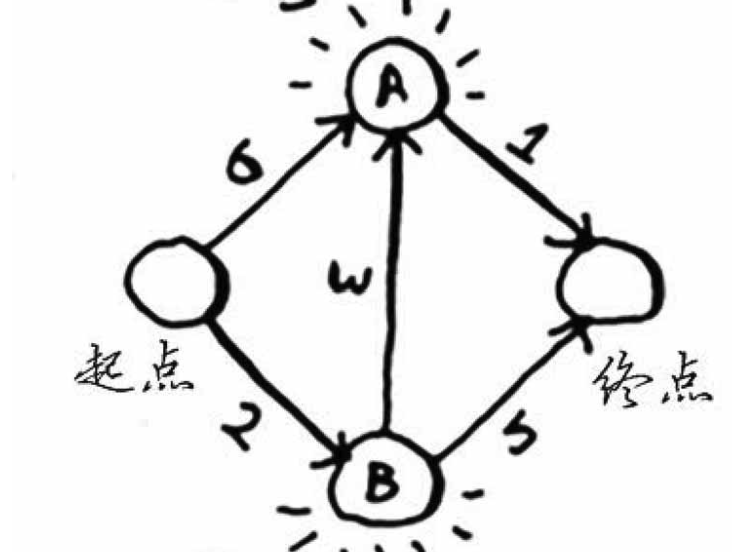
step1. 找出最便宜的节点 -> B
| A | 6 |
|---|---|
| B | 2 |
| End | inf |
step2. 计算经节点B(当前最短时间可前往的节点)前往该点各个邻居所需最短时间作为开销
| A | 6 -> 5 |
|---|---|
| B | 2 |
| End | 7 |
step3. Repeat step1&2 直到对图中每个节点都处理
- 找出可在最短时间内前往的节点。由于对节点B执行了第二步,所以除了节点B,可在最短时间内前往的节点是A
- 更新节点A的所有邻居开销,发现前往终点6min
step4. 计算最终路径
2. 术语 Glossary
- 加权图(weighted graph):每条边都有关联数字的图
- 非加权图寻找最短路径 -> 广度优先搜索
- 无向图:每条边都是一个环
3. 实例:乐谱换钢琴
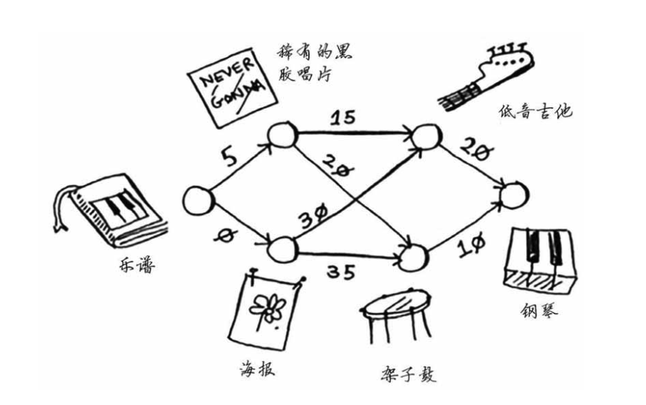
求乐谱换钢琴所需最少钱? -> Dijkstra algorithm
step0 建初始表
| 父节点 | 节点 | 开销 |
|---|---|---|
| 乐谱 | 黑胶唱片 | 5 |
| 乐谱 | 海报 | 0 |
| 吉他 | inf | |
| 架子鼓 | inf | |
| 钢琴 | inf |
step1 找出最便宜的节点 -> 海报
step2 计算前往该节点的各个邻居的开销
| 父节点 | 节点 | 开销 |
|---|---|---|
| 乐谱 | 黑胶唱片 | 5 |
| 乐谱 | 海报 | 0 |
| 海报 | 吉他 | 30 |
| 海报 | 架子鼓 | 35 |
| 钢琴 | inf |
step3 重复前两步
- 下一个最便宜的节点是黑胶唱片
- 更新黑胶唱片各个邻居的开销。由于换吉他和架子鼓的开销低于之前数值,所以替换 | 父节点 | 节点 | 开销 | | —- | —- | —- | | 乐谱 | 黑胶唱片 | 5 | | 乐谱 | 海报 | 0 | | 黑胶唱片 | 吉他 | 20 | | 黑胶唱片 | 架子鼓 | 25 | | | 钢琴 | inf |
- 再重复 -> 吉他 -> 架子鼓 | 父节点 | 节点 | 开销 | | —- | —- | —- | | 乐谱 | 黑胶唱片 | 5 | | 乐谱 | 海报 | 0 | | 黑胶唱片 | 吉他 | 20 | | 黑胶唱片 | 架子鼓 | 25 | | 吉他 | 钢琴 | 40 |
| 父节点 | 节点 | 开销 |
|---|---|---|
| 乐谱 | 黑胶唱片 | 5 |
| 乐谱 | 海报 | 0 |
| 黑胶唱片 | 吉他 | 20 |
| 黑胶唱片 | 架子鼓 | 25 |
| 架子鼓 | 钢琴 | 30 |
最后得到,我仅需要支付30美元即可交换得到钢琴。根据父节点进行回溯,便得到了完整地交换路径:
钢琴 <- 架子鼓 <- 黑胶唱片 <- 乐谱
4. 负权图
Dijkstra算法不适用,因为该算法是基于正向递增序列的,如果有负值,则会使序列上下波动。
- 假设:对于处理过的节点,没有前往该节点的更短路径。这种假设仅在没有负权边时成立
- 新算法:贝尔曼-福德算法(Bellman-Ford algorithm)
5. Dijkstra算法证明
[知乎] 大连理工大学,公式归纳证明,反证法
[youtube] 北大,归纳证明
数学归纳法
命题:算法进行到第k步时,set中每个节点从起始到节点i的距离dist[i]等于全局最短路径short[i](第n步时,可以得到dist[n]==short[n],此时找到了起始点到所有节点的距离/权重)
归纳基础:原点进入归纳集合
- k=1, set={start} -> dist[start] = short[start]=0,命题正确,没有边
- 归纳步骤:
- 如果k步成立,dist[k] == short[k]
- 那么k+1步也成立,即
证明归纳步骤(感觉不太对:没有k步成立)
- 假设命题对k为真,考虑k+1算法选择顶点v(边
- 法1. 若存在另一条s-v路径,最后一次出s顶点为x,经过v-s的第一个顶点y,再由y经过一段在v-s中的路径到达v
- 在k+1步算法选择顶点v,而不是y,即dist[v] <= dist[y](这步是第k步得出的结论,已计算出圈内已处理过节点到圈外第一层节点的距离,所以可以直接得到距离最小的节点v)
- 令y到v的路径长度为d(y,v),dist[y] + d(y,v) <=L
- 因此:dist[v] <= L,即 dist[v]=short[v]
- 反证法:
- 若存在另一条路 dist[new-v] < dist[alg_v]
- Dijkstra算法寻找的是dist[alg_v] == short[alg_v]
- 因为:dist[alg_v] <= dist[new_v]矛盾
- 所以:dist[alg_v] 是当前k+1轮找到的最短路径
- 反证法:
Wiki proof
- Proof of Dijkstra’s algorithm is constructed by induction on the number of visited nodes.
Invariant hypothesis: For each node v, dist[v] is the shortest distance from source to v when traveling via visited nodes only, or infinity if no such path exists.
The base case is when there is just one visited node, namely(that is to say) the initial node source, in which case the hypothesis is trivial.
- 注:反证法需要假定我们证明的结论是错误的,最后出现矛盾
Otherwise, assume the hypothesis for n-1 visited nodes. (v是n-1节点)In which case, we choose an edge vu where u has the least dist[u] of any unvisited nodes and the edge vu is such that dist[u] = dist[v] + length[v, u]. dist[u] is considered to be the shortest distance from source to u because if there were a shorter path, and if w was the first unvisited node on that path then by the original hypothesis dist[w] > dist[u] which creates a contradiction. Similarly if there were a shorter path to u without using unvisited nodes, and if the last but one node on that path were w, then we would have had dist[u] = dist[w] + length[w, u], also a contradiction.
After processing u it will still be true that for each unvisited node w, dist[w] will be the shortest distance from source to w using visited nodes only, because if there were a shorter path that doesn’t go by u we would have found it previously, and if there were a shorter path using u we would have updated it when processing u.
After all nodes are visited, the shortest path from source to any node v consists only of visited nodes, therefore dist[v] is the shortest distance.

若有收获,就点个赞吧
0 人点赞
