数据集简介
数据包括如下10类信息:
Clothing ID: 服装标签,数字信息
Age: 购买者年龄,数字信息
Title: 评论标题,文字信息
Review Text: 评论内容,文字信息
Rating: 产品评价(评分由低到高用0-5表示),数字信息
Recommended IND:是否推荐(0表示不推荐,1表示推荐),数字信息
Positive Feedback Count: 正面反馈数量(认为该评价有用),数字信息
Division Name: 产品分类名称,文字信息
Department Name: 服饰类别,文字信息
Class Name: 服饰类型,文字信息
Division Name包括General、General Petite和Initmates。前两者指服饰的大小,General指正常大小,General Petite指为身材娇小的女性提供的服饰,Initmates则指私人贴身服饰。Department Name包括Tops(上装)、Bottoms(下装)等区分。Class Name则是更加细致的划分。
分析主题
1、女性顾客中哪个年龄段人群是网购主力军
2、不同年龄顾客对应哪类服装
3、各类服装评价分数如何?
4、各类服装推荐情况
4、产品评价分数与是否推荐相关吗?
读取数据
#加载包import numpy as npimport pandas as pdimport matplotlib.pyplot as plt
#利用pandas导入数据clothing_df = pd.read_csv(r"C:\Users\谭小洵\Desktop\women shopping datebase\Womens Clothing E-Commerce Reviews.csv", index_col=0)
#查看数据开头clothing_df.head()
|
Clothing ID |
Age |
Title |
Review Text |
Rating |
Recommended IND |
Positive Feedback Count |
Division Name |
Department Name |
Class Name |
| 0 |
767 |
33 |
NaN |
Absolutely wonderful - silky and sexy and comf… |
4 |
1 |
0 |
Initmates |
Intimate |
Intimates |
| 1 |
1080 |
34 |
NaN |
Love this dress! it’s sooo pretty. i happene… |
5 |
1 |
4 |
General |
Dresses |
Dresses |
| 2 |
1077 |
60 |
Some major design flaws |
I had such high hopes for this dress and reall… |
3 |
0 |
0 |
General |
Dresses |
Dresses |
| 3 |
1049 |
50 |
My favorite buy! |
I love, love, love this jumpsuit. it’s fun, fl… |
5 |
1 |
0 |
General Petite |
Bottoms |
Pants |
| 4 |
847 |
47 |
Flattering shirt |
This shirt is very flattering to all due to th… |
5 |
1 |
6 |
General |
Tops |
Blouses |
数据预处理
#查看缺失值,打印表格每一列信息clothing_df.info()
<class 'pandas.core.frame.DataFrame'>Int64Index: 23486 entries, 0 to 23485Data columns (total 10 columns): # Column Non-Null Count Dtype --- ------ -------------- ----- 0 Clothing ID 23486 non-null int64 1 Age 23486 non-null int64 2 Title 19676 non-null object 3 Review Text 22641 non-null object 4 Rating 23486 non-null int64 5 Recommended IND 23486 non-null int64 6 Positive Feedback Count 23486 non-null int64 7 Division Name 23472 non-null object 8 Department Name 23472 non-null object 9 Class Name 23472 non-null objectdtypes: int64(5), object(5)memory usage: 2.0+ MB
#方法2查看缺失值clothing_df.isnull().sum()
Clothing ID 0Age 0Title 3810Review Text 845Rating 0Recommended IND 0Positive Feedback Count 0Division Name 14Department Name 14Class Name 14dtype: int64
#去掉丢失值对应的行,Division Nmae, Department Name, Class Nameclothing_df.dropna(axis=0, subset=['Division Name', 'Department Name', 'Class Name'],inplace=True)
pd.isnull(clothing_df).sum()
Clothing ID 0Age 0Title 3809Review Text 844Rating 0Recommended IND 0Positive Feedback Count 0Division Name 0Department Name 0Class Name 0dtype: int64
#将所有的缺失值替换为字符串NULLclothing_df.fillna('NULL',inplace=True)clothing_df.isnull().sum()
Clothing ID 0Age 0Title 0Review Text 0Rating 0Recommended IND 0Positive Feedback Count 0Division Name 0Department Name 0Class Name 0dtype: int64
clothing_df.describe()
|
Clothing ID |
Age |
Rating |
Recommended IND |
Positive Feedback Count |
| count |
23472.000000 |
23472.000000 |
23472.000000 |
23472.000000 |
23472.000000 |
| mean |
918.486665 |
43.200707 |
4.195552 |
0.822256 |
2.537151 |
| std |
202.727678 |
12.280913 |
1.110188 |
0.382305 |
5.703597 |
| min |
0.000000 |
18.000000 |
1.000000 |
0.000000 |
0.000000 |
| 25% |
861.000000 |
34.000000 |
4.000000 |
1.000000 |
0.000000 |
| 50% |
936.000000 |
41.000000 |
5.000000 |
1.000000 |
1.000000 |
| 75% |
1078.000000 |
52.000000 |
5.000000 |
1.000000 |
3.000000 |
| max |
1205.000000 |
99.000000 |
5.000000 |
1.000000 |
122.000000 |
在describe的结果中,年龄的均值和中位数41.00的差距不大,所以年龄分布基本符合正态分布;Rating的中位数是5.00,所以大部分消费者都给与5分(最高分)评价;Recommended IND的分位数显示该值大部分为1,所以给予推荐评价的消费者居多;Positive Feedback Count中最大值高达122,最小值为0,中位数为1,因此消费者通常不会去评价他人的反馈信息。
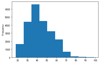
#查看年龄分布clothing_df['Age'].plot(kind='hist',bins=10)
<AxesSubplot:ylabel='Frequency'>
np.unique(clothing_df.Age[clothing_df.Age>=80],return_counts=True)
(array([80, 81, 82, 83, 84, 85, 86, 87, 89, 90, 91, 92, 93, 94, 99], dtype=int64), array([10, 5, 13, 43, 6, 6, 2, 4, 5, 2, 5, 1, 2, 3, 2], dtype=int64))
数据集中包含年龄数据。根据上面中年龄数据,虽然数据中出现超过80岁的年龄数据,但是年龄分布图呈现正态分布,因此假定所有的年龄为真实年龄。
分析
1、哪个年龄段顾客是主力军
plt.rcParams['font.sans-serif'] = ['SimHei']#设置可以显示中文plt.rcParams['axes.unicode_minus'] = False #正常显示负号
Age1 = pd.cut(clothing_df['Age'],bins=[0,18,28,38,48,58,100])age_counts=pd.value_counts(Age1)age_counts
(28, 38] 6941(38, 48] 6902(48, 58] 4114(58, 100] 3099(18, 28] 2412(0, 18] 4Name: Age, dtype: int64
plt.figure(figsize=(6,6),dpi=100)labels=['28-38岁','38-48岁','48-58岁','58-100岁','18-28岁','0-18岁']plt.pie(age_counts,autopct='%1.1f%%',labels=labels)plt.show
<function matplotlib.pyplot.show(close=None, block=None)>
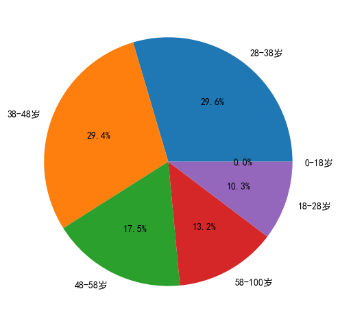
28-48岁人群占比达59%,为网购主力军
2、不同年龄顾客对应哪类服装
#根据Division Name划分clothing_df.query('0 < Age & Age <= 18').groupby('Division Name').agg( 销量 = ('Clothing ID','count')).sort_values(by='销量',ascending = False)
|
销量 |
| Division Name |
|
| General |
4 |
clothing_df.query('18 < Age & Age <= 28').groupby('Division Name').agg( 销量 = ('Clothing ID','count')).sort_values(by='销量',ascending = False)
|
销量 |
| Division Name |
|
| General |
1396 |
| General Petite |
811 |
| Initmates |
205 |
clothing_df.query('28 < Age & Age <= 38').groupby('Division Name').agg( 销量 = ('Clothing ID','count')).sort_values(by='销量',ascending = False)
|
销量 |
| Division Name |
|
| General |
4031 |
| General Petite |
2369 |
| Initmates |
541 |
clothing_df.query('38 < Age & Age <= 48').groupby('Division Name').agg( 销量 = ('Clothing ID','count')).sort_values(by='销量',ascending = False)
|
销量 |
| Division Name |
|
| General |
4130 |
| General Petite |
2392 |
| Initmates |
380 |
clothing_df.query('48 < Age & Age <= 58').groupby('Division Name').agg( 销量 = ('Clothing ID','count')).sort_values(by='销量',ascending = False)
|
销量 |
| Division Name |
|
| General |
2416 |
| General Petite |
1488 |
| Initmates |
210 |
clothing_df.query('58 < Age & Age <= 100').groupby('Division Name').agg( 销量 = ('Clothing ID','count')).sort_values(by='销量',ascending = False)
|
销量 |
| Division Name |
|
| General |
1873 |
| General Petite |
1060 |
| Initmates |
166 |
clothing_df.groupby('Division Name').agg( 销量 = ('Clothing ID','count')).sort_values(by='销量',ascending = False)
|
销量 |
| Division Name |
|
| General |
13850 |
| General Petite |
8120 |
| Initmates |
1502 |
超过18岁购物者中,均是尺寸为正常大小,稍小销量更高,可以考虑进货时多考虑这2种,三者比例大致为9:5:1。
#根据Department Name划分clothing_df.query('0 < Age & Age <= 18').groupby('Department Name').agg( 销量 = ('Clothing ID','count')).sort_values(by='销量',ascending = False)
|
销量 |
| Department Name |
|
| Dresses |
2 |
| Bottoms |
1 |
| Tops |
1 |
clothing_df.query('18 < Age & Age <= 28').groupby('Department Name').agg( 销量 = ('Clothing ID','count')).sort_values(by='销量',ascending = False)
|
销量 |
| Department Name |
|
| Tops |
995 |
| Dresses |
714 |
| Bottoms |
355 |
| Intimate |
231 |
| Jackets |
105 |
| Trend |
12 |
clothing_df.query('18 < Age & Age <= 28').groupby('Department Name').agg( 销量 = ('Clothing ID','count')).sort_values(by='销量',ascending = False)
|
销量 |
| Department Name |
|
| Tops |
995 |
| Dresses |
714 |
| Bottoms |
355 |
| Intimate |
231 |
| Jackets |
105 |
| Trend |
12 |
clothing_df.query('28 < Age & Age <= 38').groupby('Department Name').agg( 销量 = ('Clothing ID','count')).sort_values(by='销量',ascending = False)
|
销量 |
| Department Name |
|
| Tops |
2870 |
| Dresses |
1978 |
| Bottoms |
1139 |
| Intimate |
609 |
| Jackets |
314 |
| Trend |
31 |
clothing_df.query('38 < Age & Age <= 48').groupby('Department Name').agg( 销量 = ('Clothing ID','count')).sort_values(by='销量',ascending = False)
|
销量 |
| Department Name |
|
| Tops |
3073 |
| Dresses |
1897 |
| Bottoms |
1184 |
| Intimate |
457 |
| Jackets |
257 |
| Trend |
34 |
clothing_df.query('38 < Age & Age <= 48').groupby('Department Name').agg( 销量 = ('Clothing ID','count')).sort_values(by='销量',ascending = False)
|
销量 |
| Department Name |
|
| Tops |
3073 |
| Dresses |
1897 |
| Bottoms |
1184 |
| Intimate |
457 |
| Jackets |
257 |
| Trend |
34 |
clothing_df.query('48 < Age & Age <= 58').groupby('Department Name').agg( 销量 = ('Clothing ID','count')).sort_values(by='销量',ascending = False)
|
销量 |
| Department Name |
|
| Tops |
1945 |
| Dresses |
1048 |
| Bottoms |
658 |
| Intimate |
251 |
| Jackets |
184 |
| Trend |
28 |
clothing_df.query('58 < Age & Age <= 100').groupby('Department Name').agg( 销量 = ('Clothing ID','count')).sort_values(by='销量',ascending = False)
|
销量 |
| Department Name |
|
| Tops |
1584 |
| Dresses |
680 |
| Bottoms |
462 |
| Intimate |
187 |
| Jackets |
172 |
| Trend |
14 |
clothing_df.groupby('Department Name').agg( 销量 = ('Clothing ID','count')).sort_values(by='销量',ascending = False)
|
销量 |
| Department Name |
|
| Tops |
10468 |
| Dresses |
6319 |
| Bottoms |
3799 |
| Intimate |
1735 |
| Jackets |
1032 |
| Trend |
119 |
各个年龄段均已上衣,连衣裙,下装,贴身服饰为主。
#根据Class Name划分clothing_df.query('0 < Age & Age <= 18').groupby('Class Name').agg( 销量 = ('Clothing ID','count')).sort_values(by='销量',ascending = False)
|
销量 |
| Class Name |
|
| Dresses |
2 |
| Knits |
1 |
| Skirts |
1 |
clothing_df.query('18 < Age & Age <= 28').groupby('Class Name').agg( 销量 = ('Clothing ID','count')).sort_values(by='销量',ascending = False)
|
销量 |
| Class Name |
|
| Dresses |
714 |
| Knits |
478 |
| Blouses |
305 |
| Sweaters |
121 |
| Pants |
119 |
| Skirts |
103 |
| Jeans |
92 |
| Fine gauge |
91 |
| Lounge |
75 |
| Jackets |
73 |
| Swim |
57 |
| Shorts |
39 |
| Intimates |
35 |
| Outerwear |
32 |
| Sleep |
27 |
| Legwear |
20 |
| Layering |
17 |
| Trend |
12 |
| Casual bottoms |
2 |
clothing_df.query('28 < Age & Age <= 38').groupby('Class Name').agg( 销量 = ('Clothing ID','count')).sort_values(by='销量',ascending = False)
|
销量 |
| Class Name |
|
| Dresses |
1978 |
| Knits |
1417 |
| Blouses |
808 |
| Pants |
389 |
| Sweaters |
375 |
| Jeans |
337 |
| Skirts |
296 |
| Fine gauge |
270 |
| Lounge |
222 |
| Jackets |
219 |
| Swim |
160 |
| Shorts |
117 |
| Outerwear |
95 |
| Sleep |
62 |
| Legwear |
62 |
| Layering |
52 |
| Intimates |
50 |
| Trend |
31 |
| Chemises |
1 |
clothing_df.query('38 < Age & Age <= 48').groupby('Class Name').agg( 销量 = ('Clothing ID','count')).sort_values(by='销量',ascending = False)
|
销量 |
| Class Name |
|
| Dresses |
1897 |
| Knits |
1393 |
| Blouses |
903 |
| Pants |
434 |
| Sweaters |
426 |
| Jeans |
390 |
| Fine gauge |
351 |
| Skirts |
272 |
| Lounge |
189 |
| Jackets |
179 |
| Shorts |
88 |
| Swim |
85 |
| Outerwear |
78 |
| Sleep |
70 |
| Legwear |
41 |
| Layering |
37 |
| Intimates |
35 |
| Trend |
34 |
clothing_df.query('48 < Age & Age <= 58').groupby('Class Name').agg( 销量 = ('Clothing ID','count')).sort_values(by='销量',ascending = False)
|
销量 |
| Class Name |
|
| Dresses |
1048 |
| Knits |
843 |
| Blouses |
605 |
| Sweaters |
271 |
| Pants |
249 |
| Fine gauge |
226 |
| Jeans |
198 |
| Skirts |
161 |
| Lounge |
125 |
| Jackets |
116 |
| Outerwear |
68 |
| Shorts |
50 |
| Sleep |
35 |
| Swim |
30 |
| Trend |
28 |
| Layering |
25 |
| Legwear |
19 |
| Intimates |
17 |
clothing_df.query('58 < Age & Age <= 100').groupby('Class Name').agg( 销量 = ('Clothing ID','count')).sort_values(by='销量',ascending = False)
|
销量 |
| Class Name |
|
| Knits |
711 |
| Dresses |
680 |
| Blouses |
476 |
| Sweaters |
235 |
| Pants |
197 |
| Fine gauge |
162 |
| Jeans |
130 |
| Jackets |
117 |
| Skirts |
112 |
| Lounge |
80 |
| Outerwear |
55 |
| Sleep |
34 |
| Legwear |
23 |
| Shorts |
23 |
| Swim |
18 |
| Intimates |
17 |
| Layering |
15 |
| Trend |
14 |
各个年龄段位于前三位销量均为连衣裙、针织衫、衬衫。
3、各类服装评价分数如何?
#根据Division Name划分clothing_df.groupby('Division Name').agg( 评价分数 = ('Rating','mean')).sort_values(by='评价分数',ascending = False)
|
评价分数 |
| Division Name |
|
| Initmates |
4.286285 |
| General Petite |
4.211084 |
| General |
4.176606 |
#根据Department Name划分clothing_df.groupby('Department Name').agg( 评价分数 = ('Rating','mean')).sort_values(by='评价分数',ascending = False)
|
评价分数 |
| Department Name |
|
| Bottoms |
4.288760 |
| Intimate |
4.280115 |
| Jackets |
4.264535 |
| Tops |
4.172239 |
| Dresses |
4.150815 |
| Trend |
3.815126 |
#根据Class Name划分clothing_df.groupby('Class Name').agg( 评价分数 = ('Rating','mean')).sort_values(by='评价分数',ascending = False)
|
评价分数 |
| Class Name |
|
| Casual bottoms |
4.500000 |
| Layering |
4.376712 |
| Jeans |
4.360942 |
| Lounge |
4.301013 |
| Jackets |
4.295455 |
| Sleep |
4.285088 |
| Intimates |
4.279221 |
| Legwear |
4.278788 |
| Pants |
4.265850 |
| Fine gauge |
4.260909 |
| Shorts |
4.255521 |
| Skirts |
4.245503 |
| Outerwear |
4.198171 |
| Swim |
4.197143 |
| Sweaters |
4.179272 |
| Knits |
4.161677 |
| Blouses |
4.154020 |
| Dresses |
4.150815 |
| Chemises |
4.000000 |
| Trend |
3.815126 |
评分分为1-5分,整体上均有4分,可以说产品整体而言均不错。
4、各类服装推荐情况
#根据Division Name划分clothing_df.groupby('Division Name').agg( 推荐分数 = ('Recommended IND','mean')).sort_values(by='推荐分数',ascending = False)
|
推荐分数 |
| Division Name |
|
| Initmates |
0.852197 |
| General Petite |
0.825985 |
| General |
0.816823 |
#根据Department Name划分clothing_df.groupby('Department Name').agg( 推荐分数 = ('Recommended IND','mean')).sort_values(by='推荐分数',ascending = False)
|
推荐分数 |
| Department Name |
|
| Bottoms |
0.851277 |
| Intimate |
0.850144 |
| Jackets |
0.836240 |
| Tops |
0.815151 |
| Dresses |
0.808197 |
| Trend |
0.739496 |
#根据Class Name划分clothing_df.groupby('Class Name').agg( 推荐分数 = ('Recommended IND','mean')).sort_values(by='推荐分数',ascending = False)
|
推荐分数 |
| Class Name |
|
| Chemises |
1.000000 |
| Casual bottoms |
1.000000 |
| Layering |
0.883562 |
| Jeans |
0.881430 |
| Legwear |
0.860606 |
| Lounge |
0.859624 |
| Intimates |
0.857143 |
| Sleep |
0.855263 |
| Skirts |
0.845503 |
| Jackets |
0.845170 |
| Shorts |
0.839117 |
| Fine gauge |
0.837273 |
| Pants |
0.832853 |
| Knits |
0.817675 |
| Outerwear |
0.817073 |
| Blouses |
0.810139 |
| Dresses |
0.808197 |
| Swim |
0.805714 |
| Sweaters |
0.800420 |
| Trend |
0.739496 |
clothing_df.groupby('Class Name').agg( 销量合计 = ('Clothing ID','sum')).sort_values(by='销量合计',ascending = False)
|
销量合计 |
| Class Name |
|
| Dresses |
6871680 |
| Knits |
4200953 |
| Blouses |
2576796 |
| Pants |
1441937 |
| Sweaters |
1334383 |
| Jeans |
1179731 |
| Fine gauge |
991525 |
| Skirts |
950642 |
| Jackets |
686557 |
| Outerwear |
364718 |
| Lounge |
341630 |
| Swim |
145350 |
| Shorts |
137723 |
| Trend |
105554 |
| Sleep |
71607 |
| Layering |
62661 |
| Intimates |
59370 |
| Legwear |
35793 |
| Casual bottoms |
99 |
| Chemises |
10 |
各类服装评分整体约为0.8,也就是说每卖出一件商品大约有80%的概率会认为它值得推荐,产品选品还是不错的。
5、相关性矩阵
df1 = clothing_df.copy()df1.head()
|
Clothing ID |
Age |
Title |
Review Text |
Rating |
Recommended IND |
Positive Feedback Count |
Division Name |
Department Name |
Class Name |
| 0 |
767 |
33 |
NULL |
Absolutely wonderful - silky and sexy and comf… |
4 |
1 |
0 |
Initmates |
Intimate |
Intimates |
| 1 |
1080 |
34 |
NULL |
Love this dress! it’s sooo pretty. i happene… |
5 |
1 |
4 |
General |
Dresses |
Dresses |
| 2 |
1077 |
60 |
Some major design flaws |
I had such high hopes for this dress and reall… |
3 |
0 |
0 |
General |
Dresses |
Dresses |
| 3 |
1049 |
50 |
My favorite buy! |
I love, love, love this jumpsuit. it’s fun, fl… |
5 |
1 |
0 |
General Petite |
Bottoms |
Pants |
| 4 |
847 |
47 |
Flattering shirt |
This shirt is very flattering to all due to th… |
5 |
1 |
6 |
General |
Tops |
Blouses |
df2 = df1.corr(method='pearson')df2
|
Clothing ID |
Age |
Rating |
Recommended IND |
Positive Feedback Count |
| Clothing ID |
1.000000 |
0.017322 |
-0.017626 |
-0.015414 |
0.045875 |
| Age |
0.017322 |
1.000000 |
0.026967 |
0.030712 |
0.043049 |
| Rating |
-0.017626 |
0.026967 |
1.000000 |
0.792311 |
-0.064820 |
| Recommended IND |
-0.015414 |
0.030712 |
0.792311 |
1.000000 |
-0.068954 |
| Positive Feedback Count |
0.045875 |
0.043049 |
-0.064820 |
-0.068954 |
1.000000 |
import matplotlib as mplimport seaborn as sns
plt.figure(figsize=(10,6),dpi=100)sns.heatmap(df2,xticklabels=df2.columns,yticklabels=df2.columns,cmap='RdBu',center=-1,annot=True)plt.title('购物反馈相关性矩阵',fontsize=22)plt.xticks(fontsize=12, rotation=45, horizontalalignment='right')plt.yticks(fontsize=12)
(array([0.5, 1.5, 2.5, 3.5, 4.5]), [Text(0, 0.5, 'Clothing ID'), Text(0, 1.5, 'Age'), Text(0, 2.5, 'Rating'), Text(0, 3.5, 'Recommended IND'), Text(0, 4.5, 'Positive Feedback Count')])
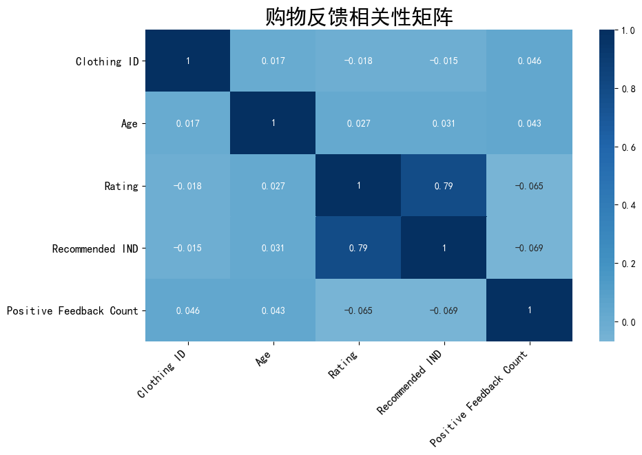
图中可以看出Rating(产品评价)和Recommended IND(是否推荐)相关性较高,可多加关注这两个指标,有利于自家产品通过消费者自发传播。
总结
1、女性网购主要集中在28-48岁。2、上衣,连衣裙,下装,贴身服饰可以多进货,三者比例可根据过往做个大致推断,尺寸则以正常大小及稍小为主,连衣裙、针织衫、衬衫购买者较多。3、产品选品整体不错。4、产品评价和是否推荐相关性较高。

