1. 为什么使用radian
适合没有窗口界面下,编辑R语言的地方,比如不能使用RStudio,然后又想用更好的编辑器(相对于R自带的编辑器),那就试试这款21世纪的R语言编辑器—radian
1. 安装radian
首先,要使用radian作为你的R语言编辑器,你要有Python3。
然后运行下面命令:
pip install -U radian
2. radian初体验
在终端下,输入radian,然后进入交互界面: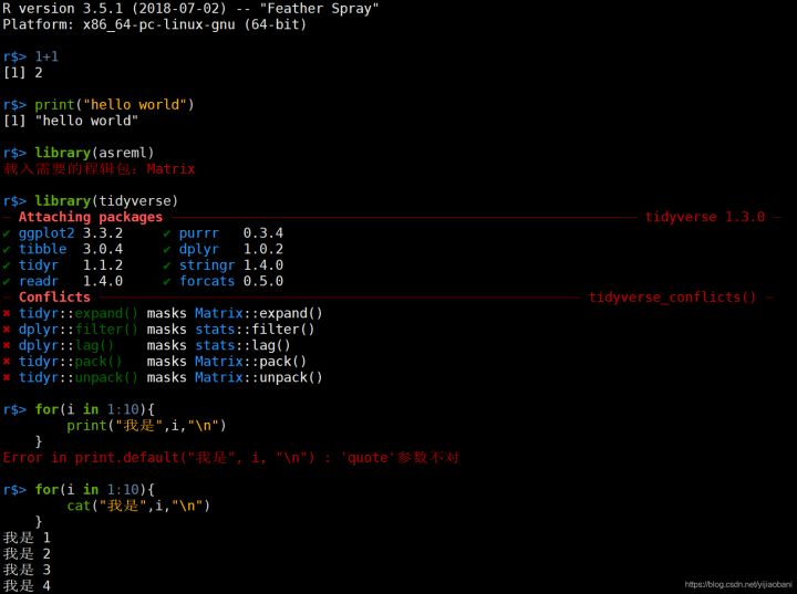
可以看到,radian界面非常漂亮,高亮语法,语法提示非常丰富,编写代码非常流畅。
2.R data frame 和 柱状图
1. Read excel files
library(readxl)A <- read_xlsx("/media/yiran/52C3-E825/qPCR/HCT116-Doxo 24h-different day/Result_table.xlsx")
快速显示绝对路径:可以直接将文件拖拽到terminal
2. Date slice
head(A[1:3,]) #数据处理前先看一下是否导入成功dim(A)colnames(A)rownames(A)
输出结果:
# A tibble: 3 × 10...1 gapdh rpl30 `b-actin` sat1 sat4 `sat13-21` D18Z1 D19Z5 D21Z1<chr> <dbl> <dbl> <dbl> <dbl> <dbl> <dbl> <dbl> <dbl> <dbl>1 M 1 1 1 1 1 1 1 1 12 D-2d 8.95 0.755 132. 49.3 11.5 52.6 77.4 0.576 59.93 D-4d 0.504 1.04 0.000381 8.94 0.157 81.9 182. 0.650 8.44[1] 20 10[1] "...1" "gapdh" "rpl30" "b-actin" "sat1" "sat4"[7] "sat13-21" "D18Z1" "D19Z5" "D21Z1"[1] "1" "2" "3" "4" "5" "6" "7" "8" "9" "10" "11" "12" "13" "14" "15"[16] "16" "17" "18" "19" "20"
change colname
colnames(A)[1]<-"time_points" #给第一列换个列名colnames(A)
[1] "time points" "gapdh" "rpl30" "b-actin" "sat1" [6] "sat4" "sat13-21" "D18Z1" "D19Z5" "D21Z1"
melt():wide 数据变long 数据
library(reshape2)head(melt(A,id.vars =c( "time","time_points")))
time time points variable value 1 1 M gapdh 1.0000000 2 1 D-2d gapdh 8.9530795 3 1 D-4d gapdh 0.5041311 4 1 D-6d gapdh 1.0393755 5 1 D-7d gapdh 0.7326901 6 2 M gapdh 1.0000000
解释:如果只提供其中一个(id.var或measure.vars), melt将假定数据集中的未指定的其余变量属于另一个变量(即若只指定了id.var的对象,其余变量属于measure.vars),如果不提供,melt将假设因素和字符变量是id variables,并且所有其他的是measured variables
结果对比:
head(melt(A))
Using time points as id variables time points variable value 1 M gapdh 1.0000000 2 D-2d gapdh 8.9530795 3 D-4d gapdh 0.5041311 4 D-6d gapdh 1.0393755 5 D-7d gapdh 0.7326901 6 M gapdh 1.0000000
将melt结果赋给Raw_A
head(Raw_A<-melt(A,id.vars =c( "time","time_points")))
time time points variable value 1 1 M gapdh 1.0000000 2 1 D-2d gapdh 8.9530795 3 1 D-4d gapdh 0.5041311 4 1 D-6d gapdh 1.0393755 5 1 D-7d gapdh 0.7326901 6 2 M gapdh 1.0000000
reshape():long 数据变wide 数据
Raw_A_bar <- reshape(Raw_A,timevar="time",idvar=c("time points","variable"), direction="wide")head(Raw_A_bar)
time points variable value.1 value.2 value.3 value.4 1 M gapdh 1.0000000 1.000000 1.000000000 1.00000000 2 D-2d gapdh 8.9530795 652.125012 0.798110124 0.05478458 3 D-4d gapdh 0.5041311 10.855766 0.008592643 0.91906370 4 D-6d gapdh 1.0393755 99.793432 0.012264976 0.17010777 5 D-7d gapdh 0.7326901 2.698721 0.009385767 0.17321759 21 M rpl30 1.0000000 1.000000 1.000000000 1.00000000
注释:
1.idvar即不进行整合的数据
2.timevar即value整合的依据,在这里即按time
3.direction选wide,即long sheet变为wide sheet
reshape 小练习
head(A)colnames(A)A_melt <- melt(A, id.vars=c("time", "time points"))head(A_melt)
# head(A)# A tibble: 6 × 11`time points` gapdh rpl30 `b-actin` sat1 sat4 `sat13-21` D18Z1 D19Z5<chr> <dbl> <dbl> <dbl> <dbl> <dbl> <dbl> <dbl> <dbl>1 M 1 1 1 1 1 1 1 12 D-2d 8.95 0.755 132. 49.3 11.5 52.6 77.4 0.5763 D-4d 0.504 1.04 0.000381 8.94 0.157 81.9 182. 0.6504 D-6d 1.04 1.33 0.000533 33.7 0.789 131. 84.5 0.6335 D-7d 0.733 0.499 0.561 0.422 0.0106 17.0 209. 0.9346 M 1 1 1 1 1 1 1 1# colnames(A)# … with 2 more variables: D21Z1 <dbl>, time <dbl>[1] "time points" "gapdh" "rpl30" "b-actin" "sat1"[6] "sat4" "sat13-21" "D18Z1" "D19Z5" "D21Z1"[11] "time"Using time points as id variables# head(A_melt)time time points variable value1 1 M gapdh 1.00000002 1 D-2d gapdh 8.95307953 1 D-4d gapdh 0.50413114 1 D-6d gapdh 1.03937555 1 D-7d gapdh 0.73269016 2 M gapdh 1.0000000
Now, let’s turn it back to raw A
A_raw = reshape(A_melt, idvar=c("time", "time points"),timevar="variable", direction ="wide")head(A_raw)
time time points value.gapdh value.rpl30 value.b-actin value.sat11 1 M 1.0000000 1.0000000 1.000000e+00 1.00000002 1 D-2d 8.9530795 0.7546758 1.322254e+02 49.31884133 1 D-4d 0.5041311 1.0409545 3.811148e-04 8.93856354 1 D-6d 1.0393755 1.3343924 5.333806e-04 33.66298025 1 D-7d 0.7326901 0.4987871 5.612642e-01 0.42230146 2 M 1.0000000 1.0000000 1.000000e+00 1.0000000value.sat4 value.sat13-21 value.D18Z1 value.D19Z5 value.D21Z11 1.00000000 1.00000 1.00000 1.0000000 1.0000002 11.52409058 52.56483 77.40971 0.5763165 59.9375363 0.15710282 81.92012 181.57805 0.6499784 8.4433644 0.78911529 130.57763 84.54757 0.6331612 7.4162505 0.01055863 16.95505 209.12772 0.9342387 97.1647886 1.00000000 1.00000 1.00000 1.0000000 1.000000
We can turn dataframe back to the origin format with reshap() after melt(). The only problem is the colnamesare a little different from original one
3.calculate the sd/sem
library(plotrix)library(matrixStats)Raw_A_bar$Mean <- rowMeans(Raw_A_bar[,3:6])Raw_A_bar$sem <- std.error(t(Raw_A_bar[,3:6]))Raw_A_bar$sd <- rowSds(as.matrix(Raw_A_bar[,3:6]))head(Raw_A_bar)
time points variable value.1 value.2 value.3 value.4 Mean sem 1 M gapdh 1.0000000 1.000000 1.000000000 1.00000000 1.0000000 0.0000000 2 D-2d gapdh 8.9530795 652.125012 0.798110124 0.05478458 165.4827467 162.2266089 3 D-4d gapdh 0.5041311 10.855766 0.008592643 0.91906370 3.0718884 2.6012908 4 D-6d gapdh 1.0393755 99.793432 0.012264976 0.17010777 25.2537950 24.8475715 5 D-7d gapdh 0.7326901 2.698721 0.009385767 0.17321759 0.9035036 0.6181118 21 M rpl30 1.0000000 1.000000 1.000000000 1.00000000 1.0000000 0.0000000 sd 1 0.000000 2 324.453218 3 5.202582 4 49.695143 5 1.236224 21 0.000000
4. 将time points列变成factor
colnames(Raw_A_bar)[1]<-"time_points" # time points有空格,无法提取colnames(Raw_A_bar)[1]
[1] "time_points"
factor()
Raw_A_bar$time_points # 不要自己打,要复制粘帖factor(Raw_A_bar$time_points, levels = c('M', 'D-2d', 'D-4d', 'D-6d')) #先看一下对不对,再进行赋值Raw_A_bar$time_points<-factor(Raw_A_bar$time_points, levels = c('M', 'D-2d', 'D-4d', 'D-6d', "D-7d"))class(Raw_A_bar$time_points)
[1] "M" "D-2d" "D-4d" "D-6d" "D-7d" "M" "D-2d" "D-4d" "D-6d" "D-7d" "M" "D-2d" "D-4d" "D-6d" "D-7d" "M" [17] "D-2d" "D-4d" "D-6d" "D-7d" "M" "D-2d" "D-4d" "D-6d" "D-7d" "M" "D-2d" "D-4d" "D-6d" "D-7d" "M" "D-2d" [33] "D-4d" "D-6d" "D-7d" "M" "D-2d" "D-4d" "D-6d" "D-7d" "M" "D-2d" "D-4d" "D-6d" "D-7d" [1] M D-2d D-4d D-6d D-7d M D-2d D-4d D-6d D-7d M D-2d D-4d D-6d D-7d M D-2d D-4d D-6d D-7d M D-2d [23] D-4d D-6d D-7d M D-2d D-4d D-6d D-7d M D-2d D-4d D-6d D-7d M D-2d D-4d D-6d D-7d M D-2d D-4d D-6d [45] D-7d Levels: M D-2d D-4d D-6d D-7d [1] "factor"
5.画图:
geom_bar()
使用geom_bar()函数绘制条形图,条形图的高度通常表示两种情况之一:每组中的数据的个数,或数据框中列的值,高度表示的含义是由geom_bar()函数的参数stat决定的,stat在geom_bar()函数中有两个有效值:count和identity。默认情况下,stat=”count”,这意味着每个条的高度等于每组中的数据的个数,并且,它与映射到y的图形属性不相容,所以,当设置stat=”count”时,不能设置映射函数aes()中的y参数。如果设置stat=”identity”,这意味着条形的高度表示数据数据的值,而数据的值是由aes()函数的y参数决定的,就是说,把值映射到y,所以,当设置stat=”identity”时,必须设置映射函数中的y参数,把它映射到数值变量。
参数注释:
- stat:设置统计方法,有效值是count(默认值) 和 identity,其中,count表示条形的高度是变量的数量,identity表示条形的高度是变量的值;
- position:位置调整,有效值是stack、dodge和fill,默认值是stack(堆叠),是指两个条形图堆叠摆放,dodge是指两个条形图并行摆放,fill是指按照比例来堆叠条形图,每个条形图的高度都相等,但是高度表示的数量是不尽相同的。
- width:条形图的宽度,是个比值,默认值是0.9
- color:条形图的线条颜色
- fill:条形图的填充色
geom_errorbar():
其中的position=必须和geom_bar的一致,也选组dodge,括号里的宽度也必须一致,即为geom_bar的默认值0.9scale_fill_brewer():
选择颜色 ```r
ggplot(Raw_A_bar, aes(variable, Mean, fill=time_points)) +
geom_bar(stat=’identity’, position = ‘Dodge’) +
geom_errorbar(aes(ymin= Mean-sem, ymax= Mean+sem),
```r
ggplot(Raw_A_bar, aes(variable, Mean, fill=time_points)) +
geom_bar(stat=’identity’, position = ‘Dodge’) +
geom_errorbar(aes(ymin= Mean-sem, ymax= Mean+sem),
theme_bw()+ scale_fill_brewer(palette=”BrBG”)width=0.2, position=position_dodge(.9))+
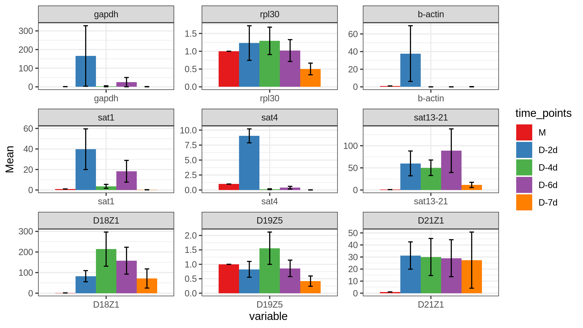
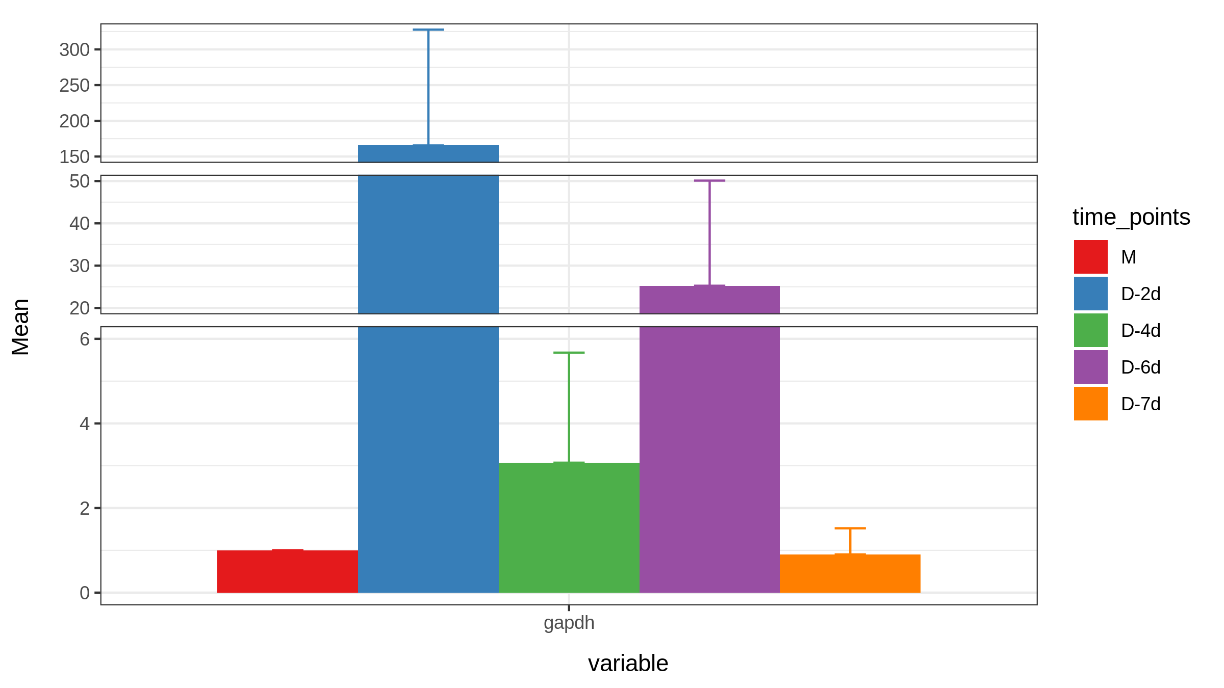
<a name="oJ1qr"></a>## 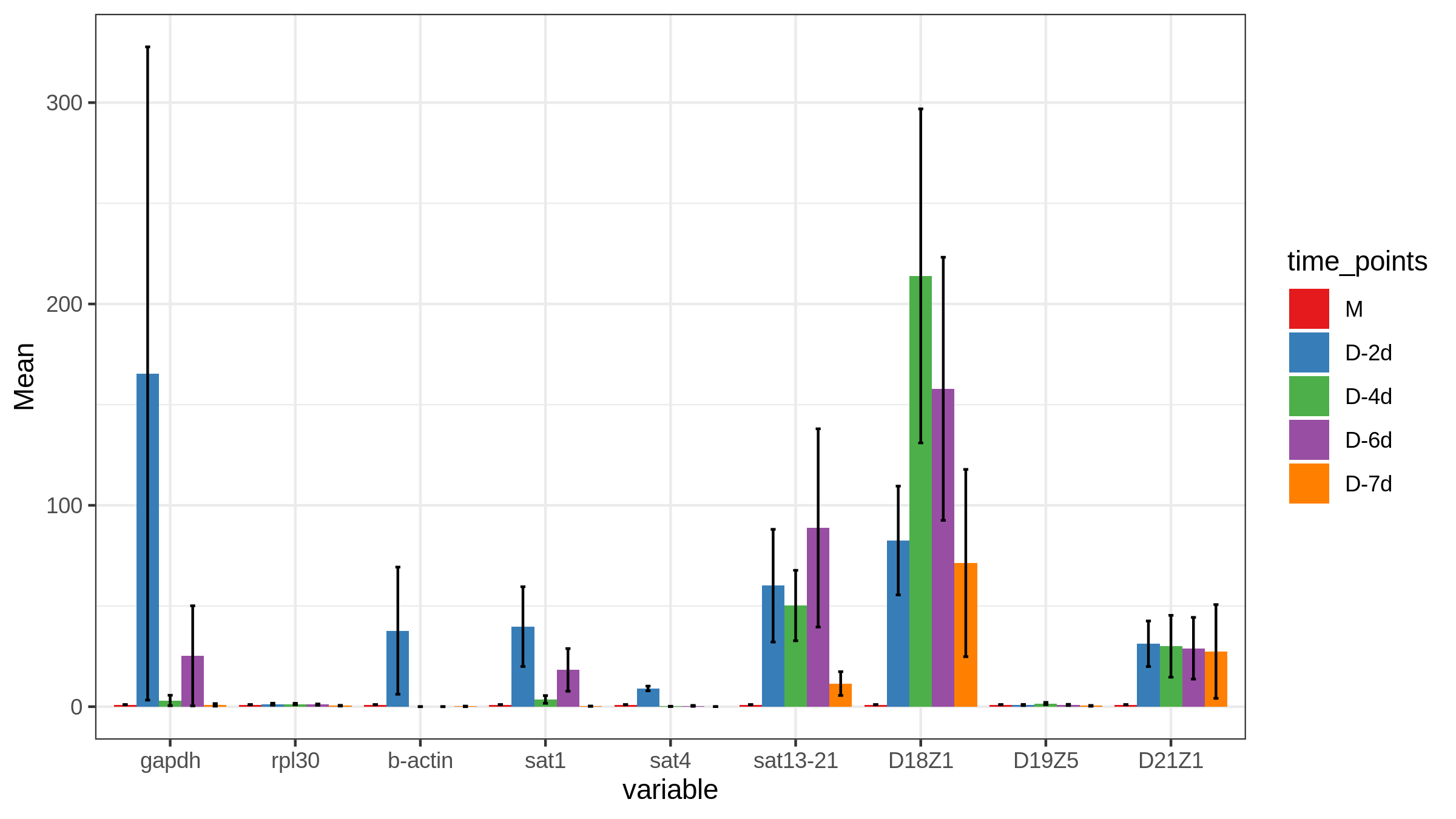```rggplot(Raw_A_bar, aes(variable, Mean, fill=time_points)) +geom_bar(stat='identity', position = 'Dodge') +geom_errorbar(aes(ymin= Mean-sem, ymax= Mean+sem),width=0.2, position=position_dodge(.9))+theme_bw()+scale_fill_brewer(palette="Set1")+facet_wrap(~ variable, scale = "free", nrow = 3)
数据切片
Raw_A_bar$variableRaw_A_bar$variable=="sat1"Raw_A_bar[Raw_A_bar$variable=="sat1",]sat1<-Raw_A_bar[Raw_A_bar$variable=="sat1",]sat1
[1] gapdh gapdh gapdh gapdh gapdh rpl30 rpl30 rpl30 rpl30 rpl30 b-actin b-actin [13] b-actin b-actin b-actin sat1 sat1 sat1 sat1 sat1 sat4 sat4 sat4 sat4 [25] sat4 sat13-21 sat13-21 sat13-21 sat13-21 sat13-21 D18Z1 D18Z1 D18Z1 D18Z1 D18Z1 D19Z5 [37] D19Z5 D19Z5 D19Z5 D19Z5 D21Z1 D21Z1 D21Z1 D21Z1 D21Z1 Levels: gapdh rpl30 b-actin sat1 sat4 sat13-21 D18Z1 D19Z5 D21Z1 [1] FALSE FALSE FALSE FALSE FALSE FALSE FALSE FALSE FALSE FALSE FALSE FALSE FALSE FALSE FALSE TRUE TRUE TRUE TRUE [20] TRUE FALSE FALSE FALSE FALSE FALSE FALSE FALSE FALSE FALSE FALSE FALSE FALSE FALSE FALSE FALSE FALSE FALSE FALSE [39] FALSE FALSE FALSE FALSE FALSE FALSE FALSE time_points variable value.1 value.2 value.3 value.4 Mean sem sd 61 M sat1 1.0000000 1.00000000 1.00000000 1.0000000 1.000000 0.00000000 0.0000000 62 D-2d sat1 49.3188413 91.50323759 14.67014446 3.5031364 39.748840 19.81748932 39.6349786 63 D-4d sat1 8.9385635 3.35044854 0.01685515 2.0293786 3.583811 1.91196379 3.8239276 64 D-6d sat1 33.6629802 39.32021348 0.01137050 0.0445459 18.259778 10.58930135 21.1786027 65 D-7d sat1 0.4223014 0.01269202 0.12645709 0.3687417 0.232548 0.09753077 0.1950615 time_points variable value.1 value.2 value.3 value.4 Mean sem sd 61 M sat1 1.0000000 1.00000000 1.00000000 1.0000000 1.000000 0.00000000 0.0000000 62 D-2d sat1 49.3188413 91.50323759 14.67014446 3.5031364 39.748840 19.81748932 39.6349786 63 D-4d sat1 8.9385635 3.35044854 0.01685515 2.0293786 3.583811 1.91196379 3.8239276 64 D-6d sat1 33.6629802 39.32021348 0.01137050 0.0445459 18.259778 10.58930135 21.1786027 65 D-7d sat1 0.4223014 0.01269202 0.12645709 0.3687417 0.232548 0.09753077 0.1950615
ggplot(sat1, aes(variable, Mean, fill=time_points)) +geom_bar(stat='identity', position = 'Dodge') +geom_errorbar(aes(ymin= Mean, ymax= Mean+sem , color=time_points),width=0.2, position=position_dodge(.9))+ theme_bw()+scale_fill_brewer(palette="Set1")+scale_color_brewer(palette = "Set1")+scale_y_break(c(6,15), scales= .5)
注:
1.若想只显示上部分error bar,只需要ymin=Mean
2.若想errorbar颜色和柱形图一致,则添加scale_color_brewer设置和scale_fill_brewer一致即可
3.scale_y_break中c(6,15),及6-15这一段是被截断的,scale即上下部分图的比例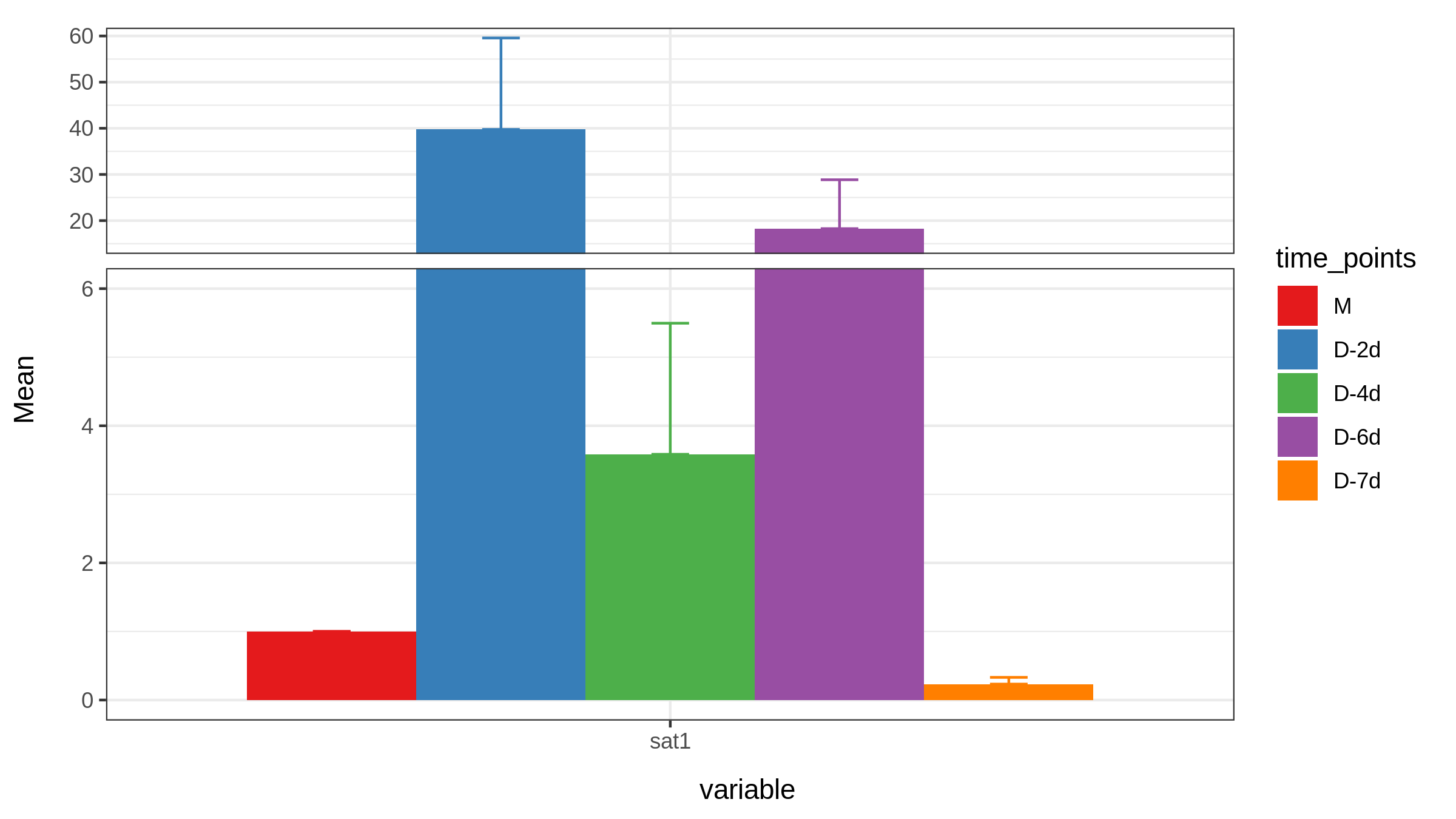 类似的,将所有数据都进行切片
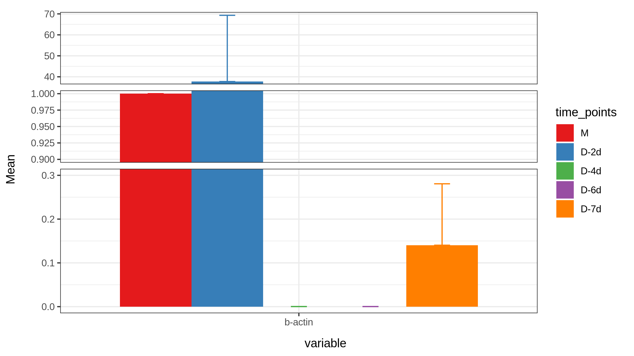
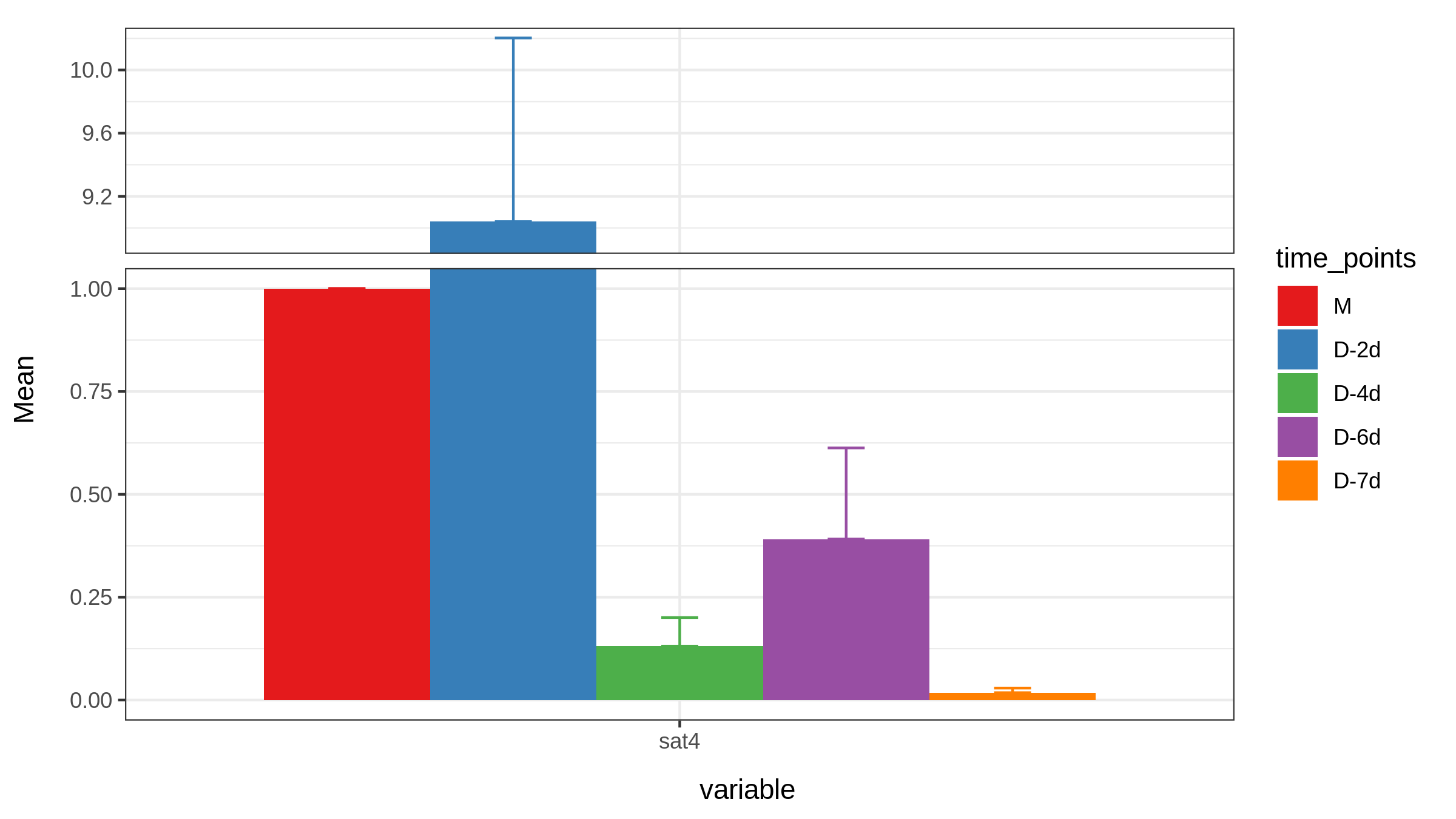
Raw_A_bar$variableRaw_A_bar$variable=="gapdh"Raw_A_bar[Raw_A_bar$variable=="gapdh",]gapdh<-Raw_A_bar[Raw_A_bar$variable=="gapdh",]gapdhP1 <- ggplot(gapdh, aes(variable, Mean, fill=time_points)) +geom_bar(stat='identity', position = 'Dodge') +geom_errorbar(aes(ymin= Mean, ymax= Mean+sem , color=time_points),width=0.2, position=position_dodge(.9))+ theme_bw()+scale_fill_brewer(palette="Set1")+scale_color_brewer(palette = "Set1")+scale_y_break(c(6,20,50,150), scales= .5)Raw_A_bar$variableRaw_A_bar$variable=="b-actin"Raw_A_bar[Raw_A_bar$variable=="b-actin",]actin<-Raw_A_bar[Raw_A_bar$variable=="b-actin",]actin # 无法用b-actin,原因同无法用空格一样P2 <- ggplot(actin, aes(variable, Mean, fill=time_points)) +geom_bar(stat='identity', position = 'Dodge') +geom_errorbar(aes(ymin= Mean, ymax= Mean+sem , color=time_points),width=0.2, position=position_dodge(.9))+ theme_bw()+scale_fill_brewer(palette="Set1")+scale_color_brewer(palette = "Set1")+scale_y_break(c(0.3,0.9,1,38), scales= .5)Raw_A_bar$variableRaw_A_bar$variable=="sat4"Raw_A_bar[Raw_A_bar$variable=="sat4",]sat4<-Raw_A_bar[Raw_A_bar$variable=="sat4",]sat4P3 <- ggplot(sat4, aes(variable, Mean, fill=time_points)) +geom_bar(stat='identity', position = 'Dodge') +geom_errorbar(aes(ymin= Mean, ymax= Mean+sem , color=time_points),width=0.2, position=position_dodge(.9))+ theme_bw()+scale_fill_brewer(palette="Set1")+scale_color_brewer(palette = "Set1")+scale_y_break(c(1,8.9), scales= .5)
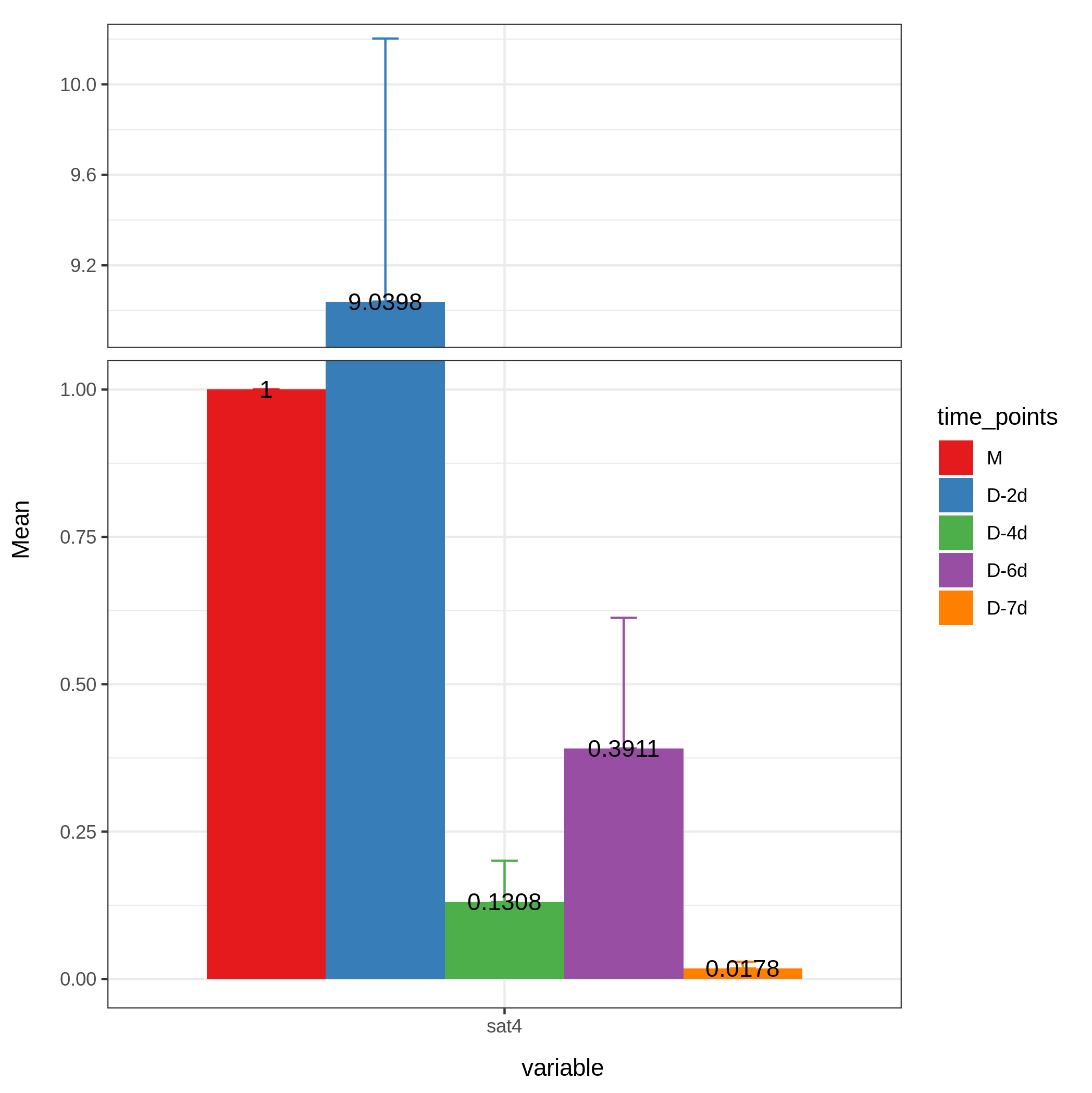
给数据加上标签:
ggplot(sat4, aes(variable, Mean, fill=time_points)) +geom_bar(stat='identity', position = 'Dodge') +geom_errorbar(aes(ymin= Mean, ymax= Mean+sem , color=time_points),width=0.2, position=position_dodge(.9))+ theme_bw()+scale_fill_brewer(palette="Set1")+scale_color_brewer(palette = "Set1")+scale_y_break(c(1,8.9), scales= .5)+geom_text(aes(y=Mean*1,label=round(Mean,4)),position=position_dodge(.9))
将数据放到一张图
library(pathwork)GGlay = "AAB"P_1 <- P1 + P2 + P3 + plot_layout(design = GGlay)P_2 <- P4 + P5 + P6 + plot_layout(design = GGlay)P_3 <- P7 + P8 + P9 + plot_layout(design = GGlay)P_1/P_2/P3
一般会将其保存为pdf格式,之后用librewoffice打开,可进行数据标签的拖拽
6.保存图片
ggsave("summary.png", w= 8, h= 4.5)
则会保存在打开terminal的地方

若有收获,就点个赞吧
0 人点赞
