https://towardsdatascience.com/gamma-distribution-intuition-derivation-and-examples-55f407423840
Gamma Distribution — Intuition, Derivation, and Examples
and why does it matter?
Before setting Gamma’s two parameters _α, β_and plugging them into the formula, let’s pause for a moment and ask a few questions…
Why did we have to invent the Gamma distribution? (i.e., why does this distribution exist?)
When should Gamma distribution be used for modeling?
1. Why did we invent Gamma distribution?
Answer: To predict the wait time until future events.
Hmmm ok, but I thought that’s what the exponential distribution is for.
Then, what’s the difference between exponential distribution and gamma distribution?
The exponential distribution predicts the wait time until the very first event. The gamma distribution, on the other hand, predicts the wait time until the k-th event occurs.
2. Let’s derive the PDF of Gamma from scratch!
In our previous post, we derived the PDF of exponential distribution from the Poisson process. I highly recommend learning Poisson & Exponentialdistribution if you haven’t already done so. Understanding them well is absolutely required for understanding the Gamma well. The order of your reading should be 1. Poisson, 2. Exponential, 3. Gamma.
The derivation of the PDF of Gamma distribution is very similar to that of the exponential distribution PDF, except for one thing — it’s the wait time until the k-th event, instead of the first event.
< Notation! > T : the random variable for wait time until the k-th event
** (This is the random variable of interest!)
Event arrivals are modeled by a Poisson process with rate λ.* k : the 1st parameter of Gamma. The # of events **for which you are waiting.
- λ : the 2nd parameter of Gamma. The rate of events happening which follows the Poisson process.* P(T > t) : The probability that the waiting time until the k-th event is greater than t time units
* P(X = k in t time units) : The Poisson probability of k events occuring during t time units
As usual, in order to get the PDF, we will first find the CDF and then differentiate it.
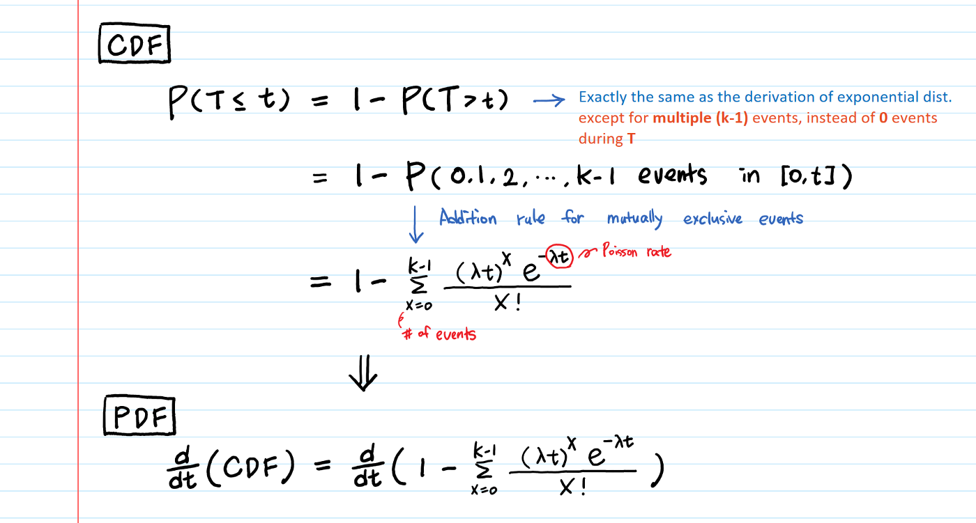
Now, let’s differentiate it.
For easier differentiation, we take out the term (e^(-λt)) when x = 0 from the summation.
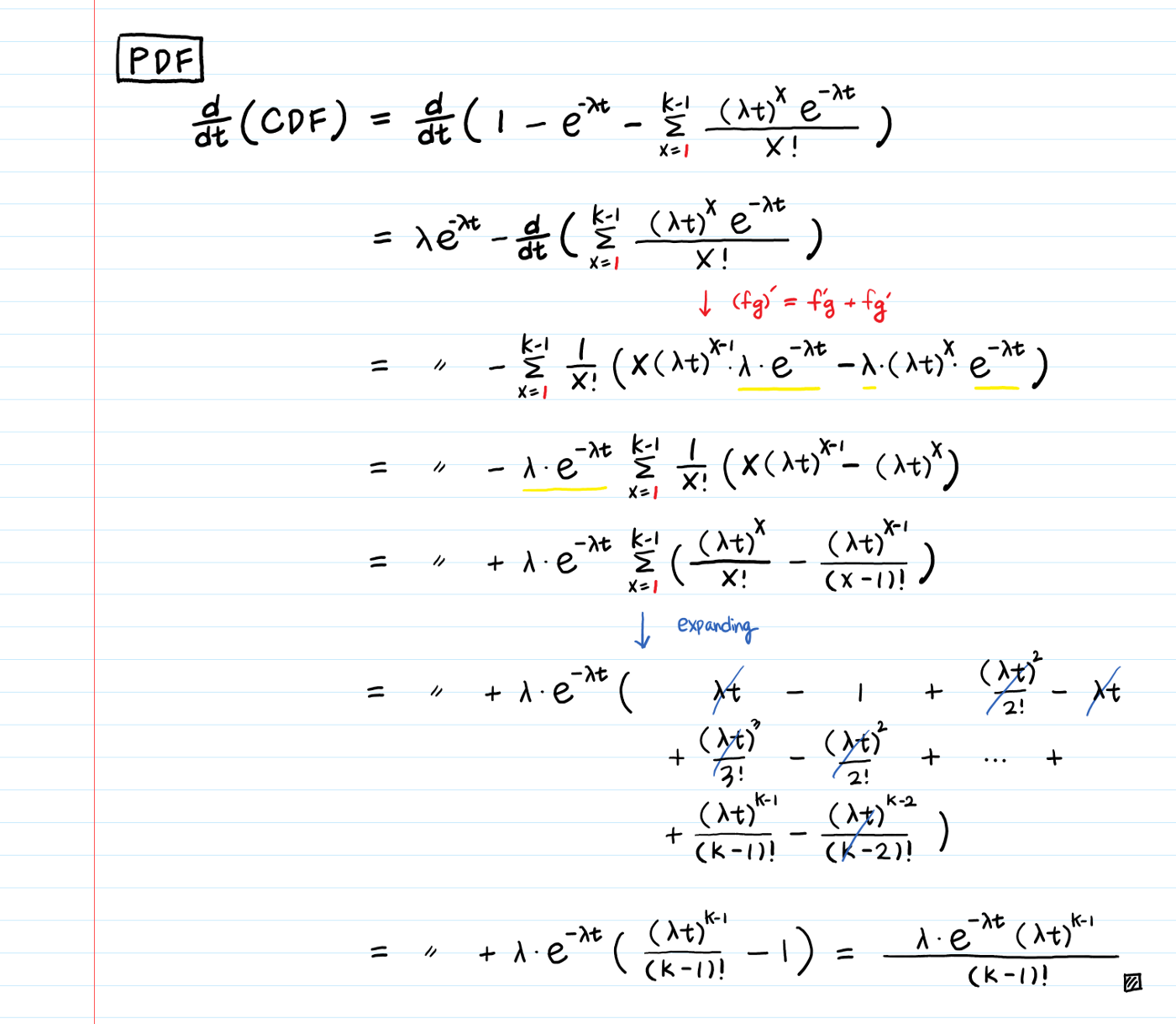
We got the PDF of gamma distribution!
The derivation looks complicated but we are merely rearranging the variables, applying the product rule of differentiation, expanding the summation, and crossing some out.
If you look at the final output of the derivation, you will notice that it is the same as the PDF of Exponential distribution, when k=1.
Since k is a positive integer (number of k events), 𝚪(k) = (k−1)! where 𝚪 denotes the gamma function. The final product can be rewritten as:
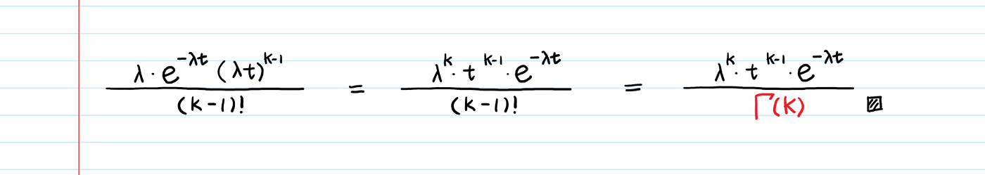
If arrivals of events follow a Poisson process with a rate λ, the wait time until k arrivals follows Γ(k, λ).
3. Parameters of Gamma: a shape or a scale?!
There are two aspects of Gamma’s parameterization that confuse us!
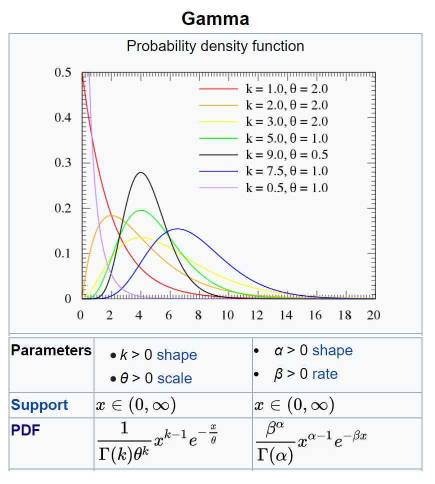
From https://en.wikipedia.org/wiki/Gamma_distribution
One is that it has two different parameterization sets — (k, θ) &(α, β) — and different forms of PDF. The other is that there is no universal consensus of what the “scale” parameter should be.
Let’s clarify this.
The first issue is pretty straightforward to clear up.
For (α, β) parameterization: Using our notation k (the # of events) & λ (the rate of events), simply substitute α with k, β with λ. The PDF stays the same format as what we’ve derived.
For (k, θ) parameterization:**θ is a reciprocal of the event rate λ**, which is the mean wait time (the average time between event arrivals).
Even though the PDFs have different formats, both parametrizations generate the same model. Just like in order to define a straight line, some use a slope and a y-intercept, while others use an x-intercept and a y-intercept, choosing one parameterization over another is a matter of taste. In my opinion, using λ as a rate parameter makes more sense, given how we derive both exponential and gamma using the Poisson rate λ. I also found (α, β) parameterization is easier to integrate.
Second, some authors call λ a scale parameter while others call θ=1/λ the scale parameter instead. IMHO, a “shape” or a “scale” parameter is really more of a misnomer. I plotted multiple Gamma PDFs with different k & λ sets (there are infinite parameter choices of k and λ, thus, there is an infinite number of possible Gamma distributions) and realized both k (and λ) change both “shape” AND “scale”. Whoever named them seriously could have given more intuitive names such as — the number of events and the Poisson rate!
Seeing is believing! Let’s visualize 🌈
Recap:k : The number of events for which you are waiting to occur.
λ : The rate of events happening which follows the Poisson process.
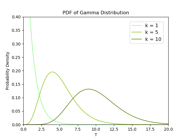
For a fixed rate λ, if we wait for more events (k) to happen, the wait time (T) will be longer.
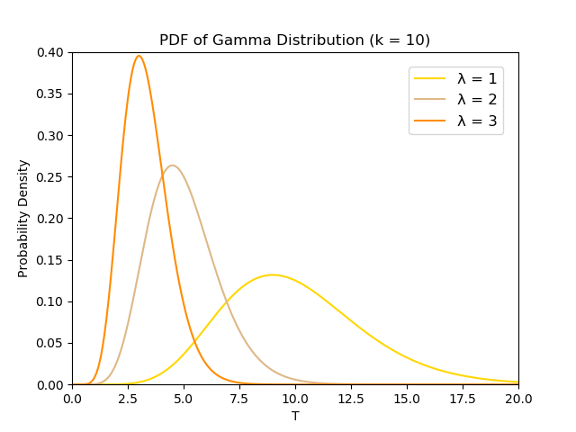
For a fixed number of events k, when the event rate λ is higher, we wait for a shorter amount of time T.
Here is Python code to generate the beautiful plots above. (Plot them yourself and see how the two parameters change the “scale” and “shape”!)
import numpy as np
from scipy.stats import gamma
import matplotlib.pyplot as pltdef plotgamma_k():
“””
k : the number of events for which you are waiting to occur.
λ : the rate of events happening following Poisson dist.
“””
x = np.linspace(0, 50, 1000)
a = 1 # k = 1
mean, var, skew, kurt = gamma.stats(a, moments=’mvsk’)
y1 = gamma.pdf(x, a)
a = 5 # k = 5
mean, var, skew, kurt = gamma.stats(a, moments=’mvsk’)
y2 = gamma.pdf(x, a)
a = 10 # k = 15
mean, var, skew, kurt = gamma.stats(a, moments=’mvsk’)
y3 = gamma.pdf(x, a)plt.title(“PDF of Gamma Distribution”)
plt.xlabel(“T”)
plt.ylabel(“Probability Density”)
plt.plot(x, y1, label=”k = 1”, color=’palegreen’)
plt.plot(x, y2, label=”k = 5”, color=’yellowgreen’)
plt.plot(x, y3, label=”k = 10”, color=’olivedrab’)
plt.legend(bbox_to_anchor=(1, 1), loc=’upper right’,
borderaxespad=1, fontsize=12)
plt.ylim([0, 0.40])
plt.xlim([0, 20])
plt.savefig(‘gamma_k.png’)
plt.clf()def plot_gamma_lambda():
“””
k : the number of events for which you are waiting to occur.
λ : the rate of events happening following Poisson dist.
“””
a = 10 # k = 10
x = np.linspace(0, 50, 1000)
lambda = 1
mean, var, skew, kurt = gamma.stats(a, scale=1/lambda, moments=’mvsk’)
y1 = gamma.pdf(x, a, scale=1/lambda)
lambda = 2
mean, var, skew, kurt = gamma.stats(a, scale=1/lambda, moments=’mvsk’)
y2 = gamma.pdf(x, a, scale=1/lambda)
lambda = 3
mean, var, skew, kurt = gamma.stats(a, scale=1/lambda, moments=’mvsk’)
y3 = gamma.pdf(x, a, scale=1/lambda)plt.title(“PDF of Gamma Distribution (k = 10)”)
plt.xlabel(“T”)
plt.ylabel(“Probability Density”)
plt.plot(x, y1, label=”λ = 1”, color=’gold’)
plt.plot(x, y2, label=”λ = 2”, color=’burlywood’)
plt.plot(x, y3, label=”λ = 3”, color=’darkorange’)
plt.legend(bbox_to_anchor=(1, 1), loc=’upper right’,
borderaxespad=1, fontsize=12)
plt.ylim([0, 0.40])
plt.xlim([0, 20])
plt.savefig(‘gamma_lambda.png’)
plt.clf()
Code in ipynb: https://github.com/aerinkim/TowardsDataScience/blob/master/Gamma%20Distribution.ipynb
4. Examples IRL🔥
We can use the Gamma distribution for every application where the exponential distribution is used — Wait time modeling, Reliability (failure) modeling, Service time modeling (Queuing Theory), etc. — because exponential distribution is a special case of Gamma distribution (just plug 1 into k).
[Queuing Theory Example] You went to Chipotle and joined a line with two people ahead of you. One is being served and the other is waiting. Their service times S1 and S2 are independent, exponential random variables with a mean of 2 minutes. (Thus the mean service rate is .5/minute__. If this “rate vs. time” concept confuses you, read this to clarify.)
What is the probability that you wait more than 5 minutes in the queue?
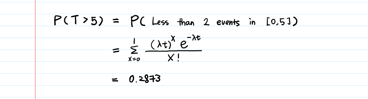
All we did was to plug t = 5 and λ = 0.5 into the CDF of the Gamma distribution that we have already derived. This is the same example that we covered in The Sum of Exponential Random Variables. As you see, we can solve this using Gamma’s CDF as well.
A less-than-30% chance that I’ll wait for more than 5 minutes at Chipotle? I’ll take that!
A few things to note:
- Poisson, Exponential, and Gamma distribution model different aspects of the same process — the Poisson process.
Poisson distribution is used to model the # of events in the future, Exponential distribution is used to predict the wait time until the very first event, and Gamma distribution is used to predict the wait time until the k-th event. - Gamma’s two parameters are both strictly positive, because one is the number of events and the other is the rate of events. They can’t be negative.
- Special cases of a Gamma distribution
╔═════════════╦══════════════════════╦══════════════════╗
║ Dist. ║ k ║ λ ║
╠═════════════╬══════════════════════╬══════════════════╣
║ Gamma ║ positive real number ║ positive real number ║
║ Exponential ║ 1 ║ “ ║
║ Erlang ║ positive integer ║ “ ║
╚═════════════╩══════════════════════╩══════════════════╝
The difference between Erlang and Gamma is that in a Gamma distribution, k can be a non-integer (positive real number) and in Erlang, k is positive integer only.
Other intuitive articles that you might like:
What is Exponential Distribution… Is the exponential parameter lambda the same as one in Poisson?…

若有收获,就点个赞吧
0 人点赞
