基于逻辑回归的分类预测
[Data Whale - 2020年8月组队打卡任务 - by Golden (wechat: freealafeimax)]
Part1 - Demo
Step1: 库函数导入
## 基础函数库import numpy as np## 导入画图库import matplotlib.pyplot as pltimport seaborn as sns## 导入逻辑回归模型函数from sklearn.linear_model import LogisticRegression
Step2: 训练模型
## Demo演示LogisticRegression分类## 构造数据集x_features = np.array([[-1,-2],[-2,-1],[-3,-2],[1,3],[2,1],[3,2]])y_label = np.array([0,0,0,1,1,1])## 调用逻辑回归模型lr_clf = LogisticRegression()## 用逻辑回归模型拟合构造的数据集lr_clf = lr_clf.fit(x_features, y_label) # 其拟合方程为 y = w0+w1*x1+w2*x2
Step3: 模型参数查看
## 查看其对应模型的wprint('The weight of Logistic Regression:', lr_clf.coef_)## 查看其对应模型的w0print('The intercept (w0) of Logistic Regression:', lr_clf.intercept_)
Output:
The weight of Logistic Regression: [[0.73462087 0.6947908 ]]
The intercept (w0) of Logistic Regression: [-0.03643213]
Step4: 数据和模型可视化
## 可视化构造的数据样本点plt.figure()plt.scatter(x_features[:,0], x_features[:,1])
Output: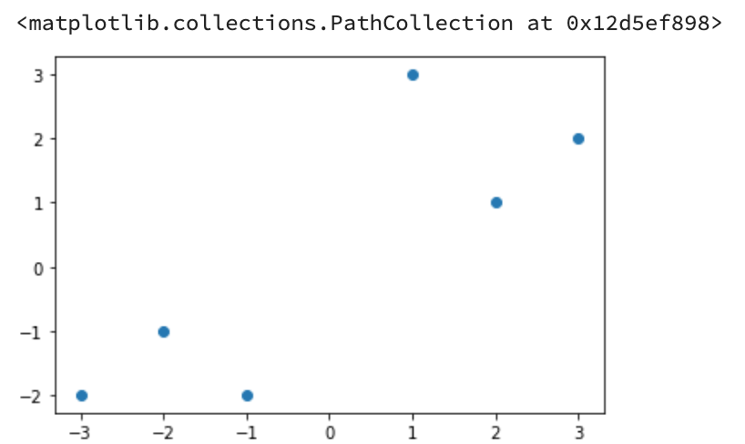
==> 为什么plt.scatter(x1, x2)中的内容是以上 (x_features[:,0], x_features[:,1]) ,查看一下:
x_features: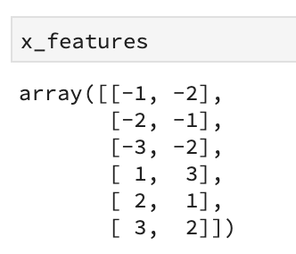
x1: 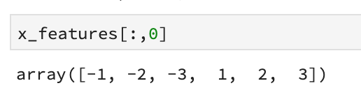
x2: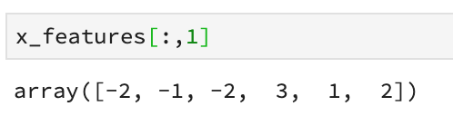
————————————————————————————————————————-
以上只是简单的散点图,下面来看看决策边界究竟如何划分:
# 可视化决策边界plt.figure()plt.scatter(x_features[:,0],x_features[:,1], c=y_label, s=50, cmap='viridis')plt.title('Dataset')nx, ny = 200, 100x_min, x_max = plt.xlim()y_min, y_max = plt.ylim()x_grid, y_grid = np.meshgrid(np.linspace(x_min, x_max, nx),np.linspace(y_min, y_max, ny))z_proba = lr_clf.predict_proba(np.c_[x_grid.ravel(), y_grid.ravel()])z_proba = z_proba[:, 1].reshape(x_grid.shape)plt.contour(x_grid, y_grid, z_proba, [0.5], linewidths=2., colors='blue')plt.show()
Output: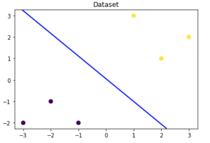
来看看matplotlib的scatter plot中的参数,即plt.scatter()内的参数:
c: 点的颜色
这里指定的是依据ylabel来定的分类的颜色,本任务的y_label有2种值,要么0,要么1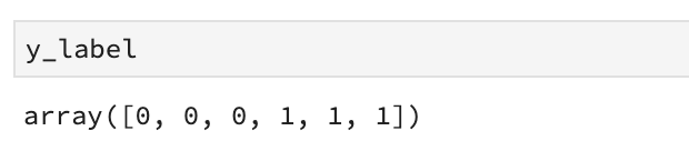 所以,就是2种颜色的点。
s: 点的大小
cmap: 点内填充颜色的选项
viridis为翡翠色中选取颜色。这里的点散点的2种颜色取自于属于viridis范畴中的2种。
[For more colors: [_https://www.taitaiblog.com/888.html](https://www.taitaiblog.com/888.html)_]_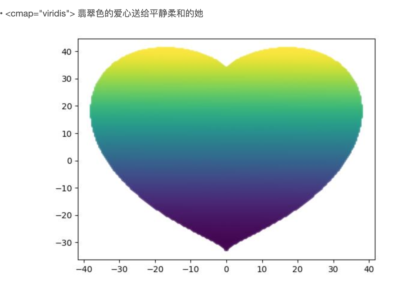
lr_clf.predict_proba()
lr_clf.predict()
这2者的区别: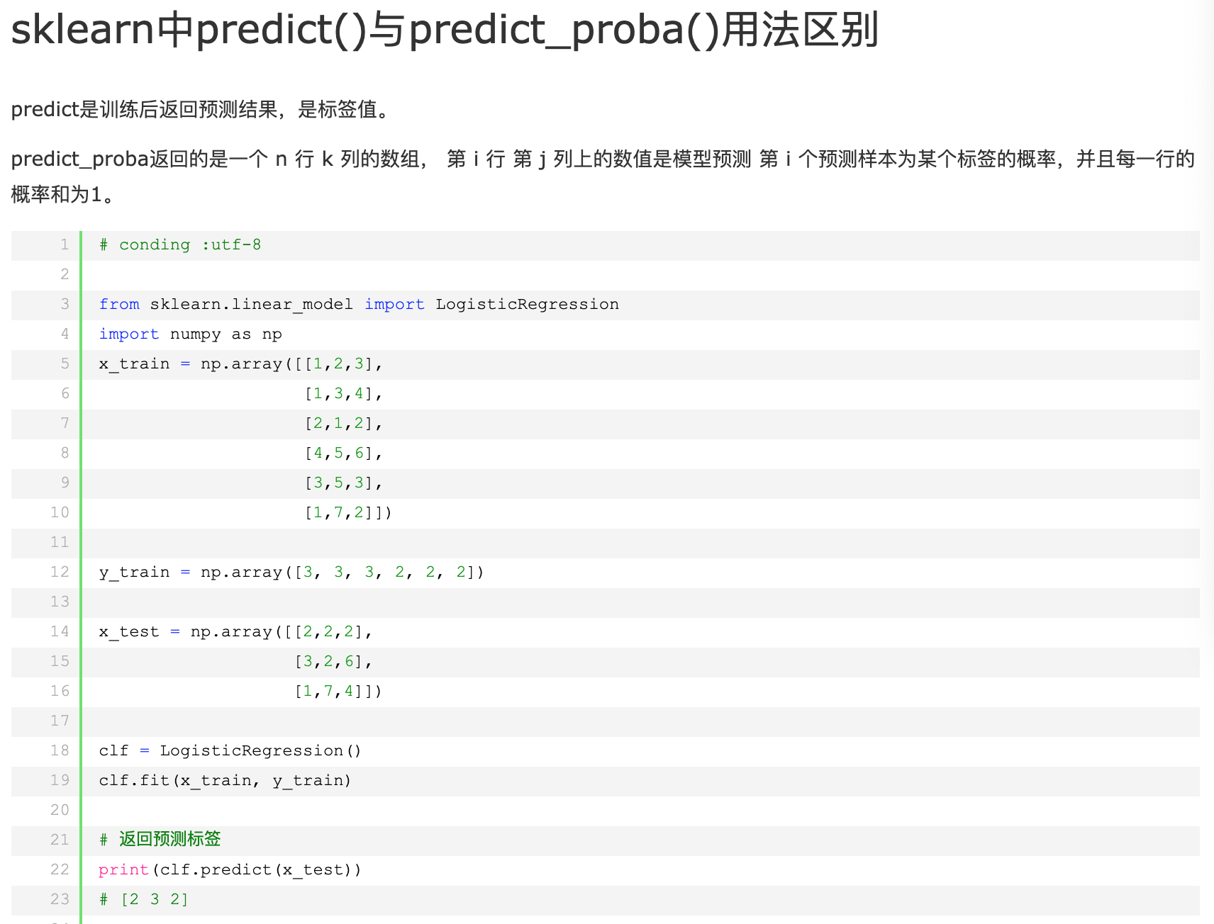
(摘自:cnblogs: https://www.cnblogs.com/mrtop/p/10309083.html)
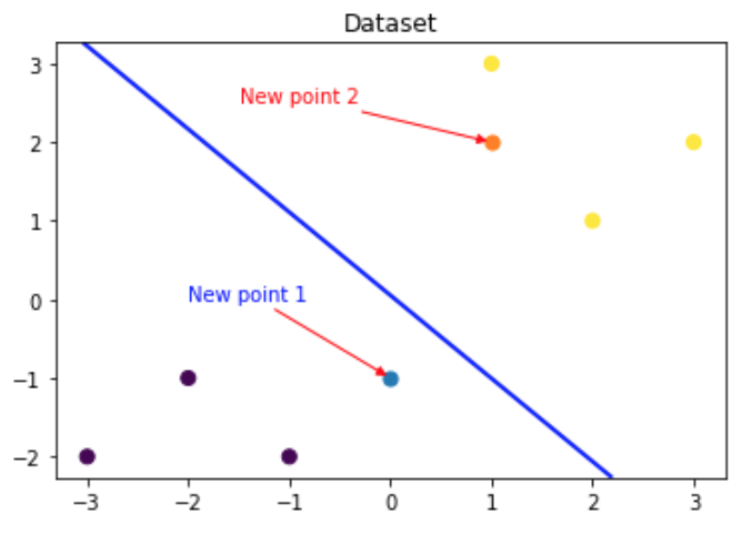
### 可视化预测新样本plt.figure()## new point 1x_features_new1 = np.array([[0, -1]])plt.scatter(x_features_new1[:,0],x_features_new1[:,1], s=50, cmap='viridis')plt.annotate(s='New point 1',xy=(0,-1),xytext=(-2,0),color='blue',arrowprops=dict(arrowstyle='-|>',connectionstyle='arc3',color='red'))## new point 2x_features_new2 = np.array([[1, 2]])plt.scatter(x_features_new2[:,0],x_features_new2[:,1], s=50, cmap='viridis')plt.annotate(s='New point 2',xy=(1,2),xytext=(-1.5,2.5),color='red',arrowprops=dict(arrowstyle='-|>',connectionstyle='arc3',color='red'))## 训练样本plt.scatter(x_features[:,0],x_features[:,1], c=y_label, s=50, cmap='viridis')plt.title('Dataset')# 可视化决策边界plt.contour(x_grid, y_grid, z_proba, [0.5], linewidths=2., colors='blue')plt.show()
Step5:模型预测
##在训练集和测试集上分布利用训练好的模型进行预测y_label_new1_predict=lr_clf.predict(x_fearures_new1)y_label_new2_predict=lr_clf.predict(x_fearures_new2)print('The New point 1 predict class:\n',y_label_new1_predict)print('The New point 2 predict class:\n',y_label_new2_predict)##由于逻辑回归模型是概率预测模型(前文介绍的p = p(y=1|x,\theta)),所有我们可以利用predict_proba函数预测其概率y_label_new1_predict_proba=lr_clf.predict_proba(x_fearures_new1)y_label_new2_predict_proba=lr_clf.predict_proba(x_fearures_new2)print('The New point 1 predict Probability of each class:\n',y_label_new1_predict_proba)print('The New point 2 predict Probability of each class:\n',y_label_new2_predict_proba)
Output: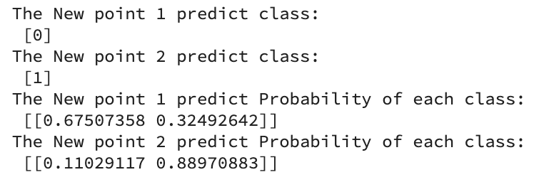
可以发现训练好的回归模型将X_new1预测为了类别0(判别面左下侧),X_new2预测为了类别1(判别面右上侧)。其训练得到的逻辑回归模型的概率为0.5的判别面为上图中蓝色的线。
Part2 - 基于鸢尾花(iris)数据集的逻辑回归分类实践
Step1:函数库导入
## 基础函数库import numpy as npimport pandas as pd## 绘图函数库import matplotlib.pyplot as pltimport seaborn as sns
本次我们选择鸢花数据(iris)进行方法的尝试训练,该数据集一共包含5个变量,其中4个特征变量,1个目标分类变量。
共有150个样本,目标变量为 花的类别 其都属于鸢尾属下的三个亚属,分别是山鸢尾 (Iris-setosa),变色鸢尾(Iris-versicolor)和维吉尼亚鸢尾(Iris-virginica)。
包含的三种鸢尾花的四个特征,分别是花萼长度(cm)、花萼宽度(cm)、花瓣长度(cm)、花瓣宽度(cm),这些形态特征在过去被用来识别物种。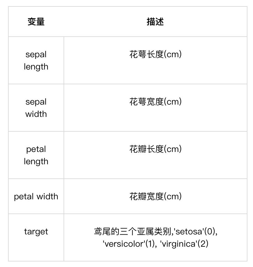
Step2: 数据读取/载入
##我们利用sklearn中自带的iris数据作为数据载入,并利用Pandas转化为DataFrame格式from sklearn.datasets import load_irisdata = load_iris() #得到数据特征iris_target = data.target #得到数据对应的标签iris_features = pd.DataFrame(data=data.data, columns=data.feature_names) #利用Pandas转化为DataFrame格式
Step3: 数据信息简单查看
iris_features.info()
Output: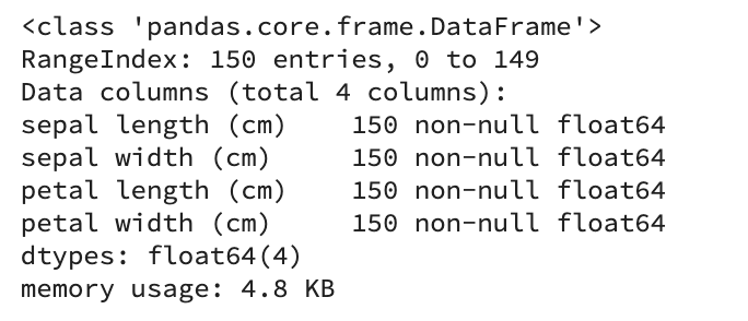
##进行简单的数据查看,我们可以利用.head()头部.tail()尾部iris_features.head()
Output: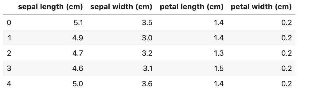
iris_features.tail()
Output: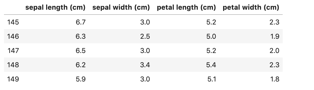
##其对应的类别标签为,其中0,1,2分别代表'setosa','versicolor','virginica'三种不同花的类别iris_target
Output: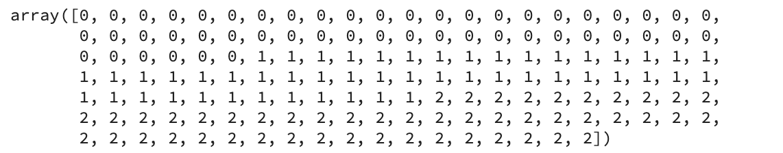
## 利用value_counts函数查看每个类别数量pd.Series(iris_target).value_counts()
Output: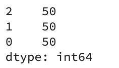
iris_target
Output: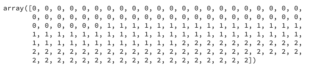
##对于特征进行一些统计描述iris_features.describe()
Output: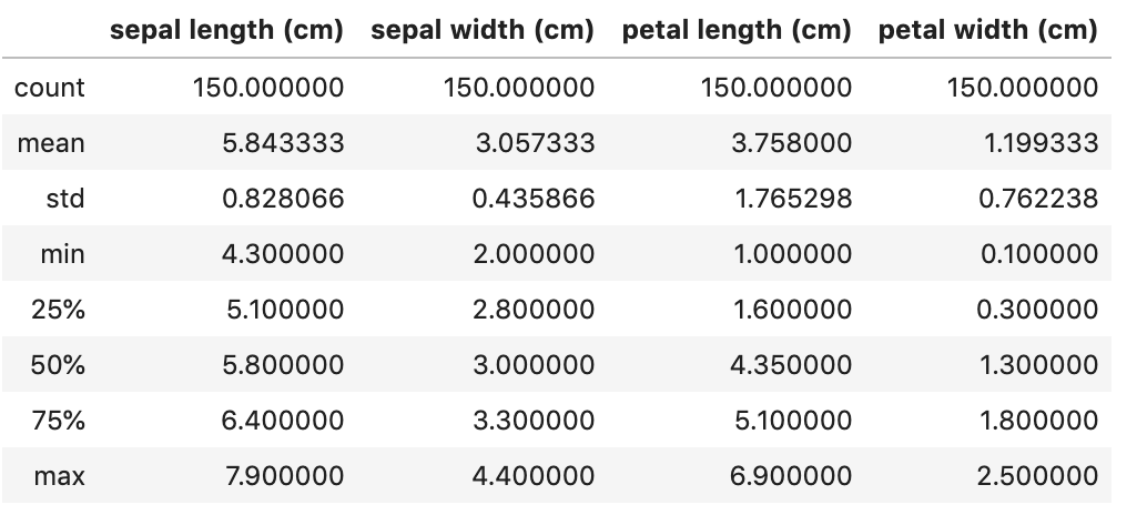
从统计描述中我们可以看到不同数值特征的变化范围。
Step4: 可视化描述
## 合并标签和特征信息iris_all = iris_features.copy() ##进行浅拷贝,防止对于原始数据的修改iris_all['target'] = iris_target
## 特征与标签组合的散点可视化sns.pairplot(data=iris_all,diag_kind='hist', hue= 'target')plt.show()
Output: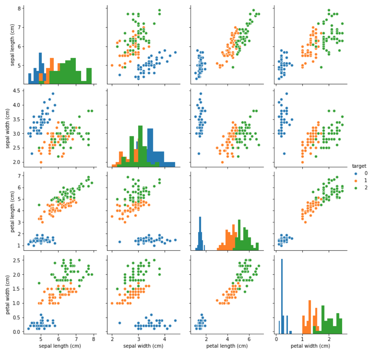
从上图可以发现,在2D情况下不同的特征组合对于不同类别的花的散点分布,以及大概的区分能力。
for col in iris_features.columns:sns.boxplot(x='target', y=col, saturation=0.5,palette='pastel', data=iris_all)plt.title(col)plt.show()
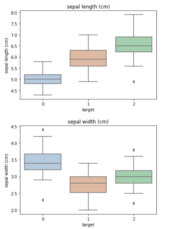
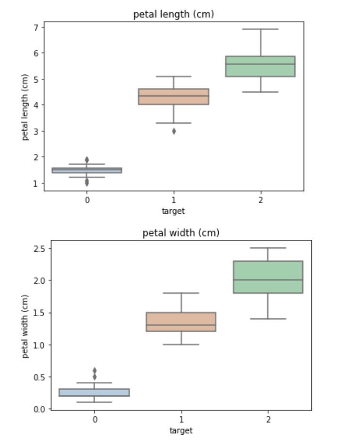
利用箱型图我们也可以得到不同类别在不同特征上的分布差异情况。
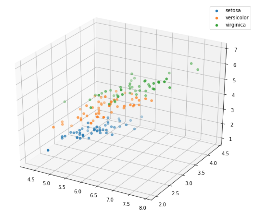
# 选取其前三个特征绘制三维散点图from mpl_toolkits.mplot3d import Axes3Dfig = plt.figure(figsize=(10,8))ax = fig.add_subplot(111, projection='3d')iris_all_class0 = iris_all[iris_all['target']==0].valuesiris_all_class1 = iris_all[iris_all['target']==1].valuesiris_all_class2 = iris_all[iris_all['target']==2].values# 'setosa'(0), 'versicolor'(1), 'virginica'(2)ax.scatter(iris_all_class0[:,0], iris_all_class0[:,1], iris_all_class0[:,2],label='setosa')ax.scatter(iris_all_class1[:,0], iris_all_class1[:,1], iris_all_class1[:,2],label='versicolor')ax.scatter(iris_all_class2[:,0], iris_all_class2[:,1], iris_all_class2[:,2],label='virginica')plt.legend()plt.show()
Step5: 利用逻辑回归在二分类上进行训练和预测
##为了正确评估模型性能,将数据划分为训练集和测试集,并在训练集上训练模型,在测试集上验证模型性能。from sklearn.model_selection import train_test_split##选择其类别为0和1的样本(不包括类别为2的样本)iris_features_part=iris_features.iloc[:100]iris_target_part=iris_target[:100]##测试集大小为20%,80%/20%分x_train,x_test,y_train,y_test=train_test_split(iris_features_part,iris_target_part,test_size=0.2,random_state=2020)
##从sklearn中导入逻辑回归模型from sklearn.linear_model import LogisticRegression
##定义逻辑回归模型clf=LogisticRegression(random_state=0,solver='lbfgs')
##在训练集上训练逻辑回归模型clf.fit(x_train,y_train)
Output: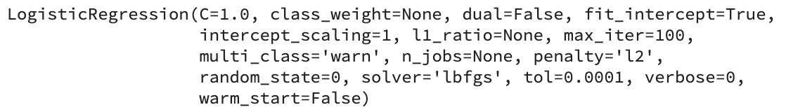
##查看其对应的wprint('the weight of Logistic Regression:',clf.coef_)##查看其对应的w0print('the intercept(w0) of Logistic Regression:',clf.intercept_)

##在训练集和测试集上分布利用训练好的模型进行预测train_predict=clf.predict(x_train)test_predict=clf.predict(x_test)
from sklearn import metrics##利用accuracy(准确度)【预测正确的样本数目占总预测样本数目的比例】评估模型效果print('The accuracy of the Logistic Regression is:',metrics.accuracy_score(y_train,train_predict))print('The accuracy of the Logistic Regression is:',metrics.accuracy_score(y_test,test_predict))##查看混淆矩阵(预测值和真实值的各类情况统计矩阵)confusion_matrix_result=metrics.confusion_matrix(test_predict,y_test)print('The confusion matrix result:\n',confusion_matrix_result)##利用热力图对于结果进行可视化plt.figure(figsize=(8,6))sns.heatmap(confusion_matrix_result,annot=True,cmap='Blues')plt.xlabel('Predictedlabels')plt.ylabel('Truelabels')plt.show()
Output: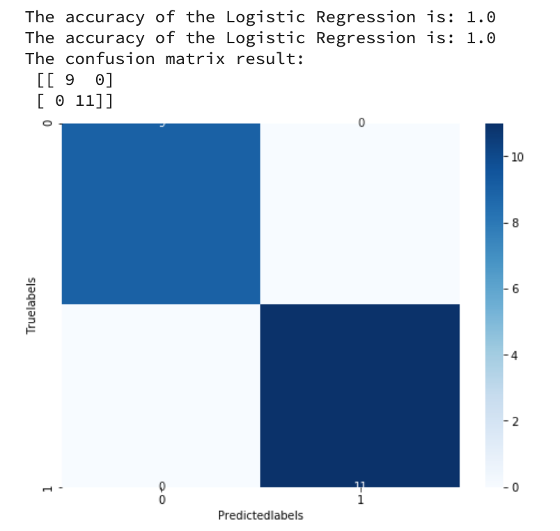
我们可以发现其准确度为1,代表所有的样本都预测正确了.
[此heatmap的第一行和最后一行被截去了一半,在后文中会解决]
Step6: 利用逻辑回归模型在三分类(多分类)上进行训练和预测
##测试集大小为20%,80%/20%分x_train,x_test,y_train,y_test=train_test_split(iris_features,iris_target,test_size=0.2,random_state=2020)
##定义逻辑回归模型clf=LogisticRegression(random_state=0,solver='lbfgs')
##在训练集上训练逻辑回归模型clf.fit(x_train,y_train)
Output: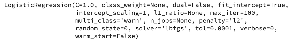
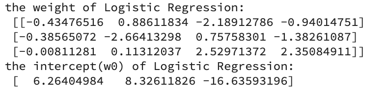
##查看其对应的wprint('the weight of Logistic Regression:\n',clf.coef_)##查看其对应的w0print('the intercept(w0) of Logistic Regression:\n',clf.intercept_)##由于这个是3分类,所有我们这里得到了三个逻辑回归模型的参数,其三个逻辑回归组合起来即可实现三分类
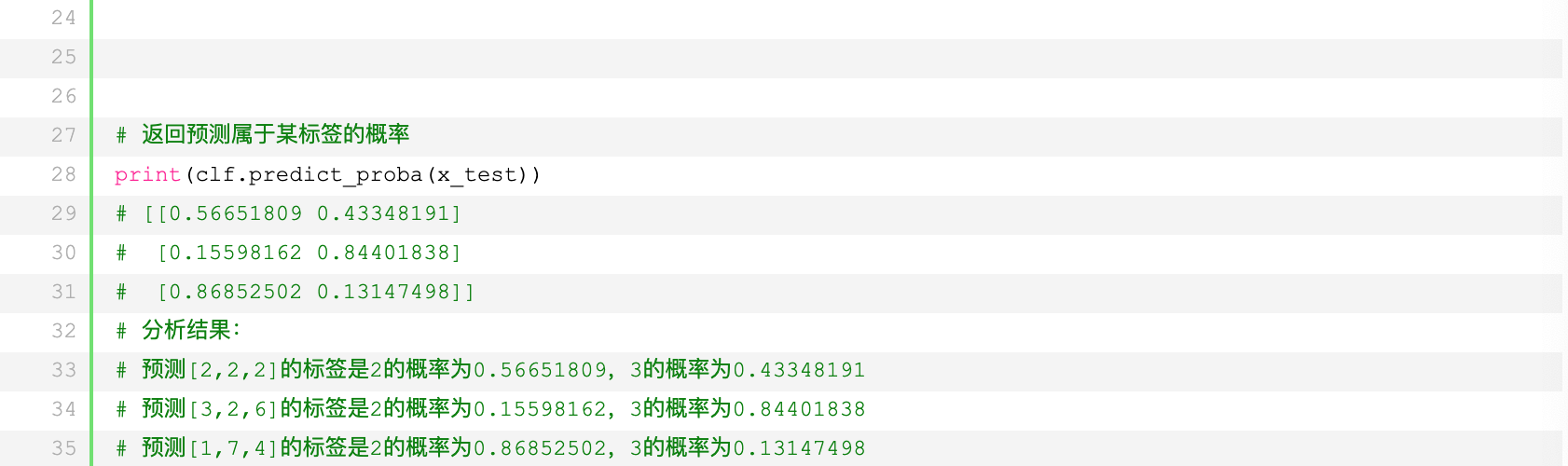
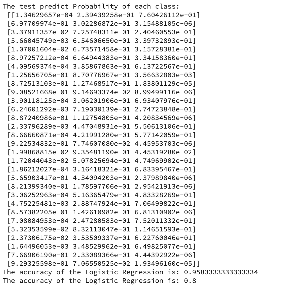
##在训练集和测试集上分布利用训练好的模型进行预测train_predict=clf.predict(x_train)test_predict=clf.predict(x_test)##由于逻辑回归模型是概率预测模型(前文介绍的p=p(y=1|x,\theta)),所有我们可以利用predict_proba函数预测其概率train_predict_proba=clf.predict_proba(x_train)test_predict_proba=clf.predict_proba(x_test)print('The test predict Probability of each class:\n',test_predict_proba)##其中第一列代表预测为0类的概率,第二列代表预测为1类的概率,第三列代表预测为2类的概率。##利用accuracy(准确度)【预测正确的样本数目占总预测样本数目的比例】评估模型效果print('The accuracy of the Logistic Regression is:',metrics.accuracy_score(y_train,train_predict))print('The accuracy of the Logistic Regression is:',metrics.accuracy_score(y_test,test_predict))
##查看混淆矩阵confusion_matrix_result=metrics.confusion_matrix(test_predict,y_test)print('The confusion matrix result:\n',confusion_matrix_result)##利用热力图对于结果进行可视化plt.figure(figsize=(8,6))sns.heatmap(confusion_matrix_result,annot=True,cmap='Blues')plt.xlabel('Predicted labels')plt.ylabel('True labels')plt.show()
Output: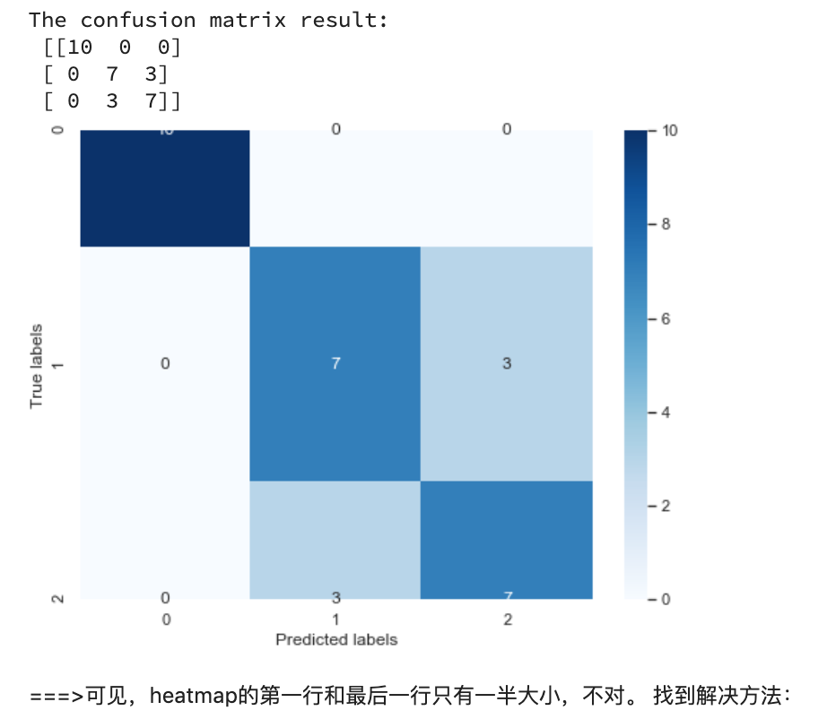
这里图形错误的原因是因为matplotlib的版本是3.1.1。
[Reference from: https://www.cnblogs.com/huanping/p/12148101.html]
方法1:
在3.1.0,3.1.2版本中都不会存在这样的问题,要么降级、升级matplotlib。
方法2:
添加一行代码,指定set_ylim的值域范围。
我们采用的是方法2,添加了:
ax.set_ylim([3, 0])
##查看混淆矩阵confusion_matrix_result=metrics.confusion_matrix(test_predict,y_test)print('The confusion matrix result:\n',confusion_matrix_result)##利用热力图对于结果进行可视化plt.figure(figsize=(8,6))ax = sns.heatmap(confusion_matrix_result,annot=True,cmap='Blues')ax.set_ylim([3, 0])plt.xlabel('Predicted labels')plt.ylabel('True labels')plt.show()
Output: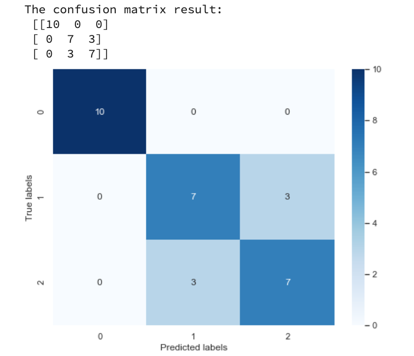
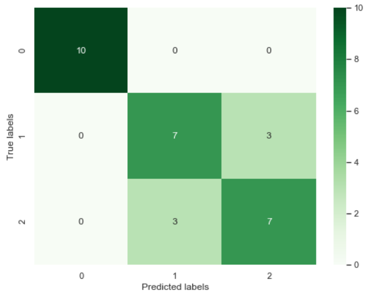
再换个绿色系的感受一下夏日清爽:
set cmap = ‘Greens’
Part3 - 逻辑回归原理简介
当z≥0 时,y≥0.5,分类为1,当 z<0时,y<0.5,分类为0,其对应的y值我们可以视为类别1的概率预测值。Logistic回归虽然名字里带“回归”,但是它实际上是一种分类方法,主要用于两分类问题(即输出只有两种,分别代表两个类别),所以利用了Logistic函数(或称为Sigmoid函数),函数形式为: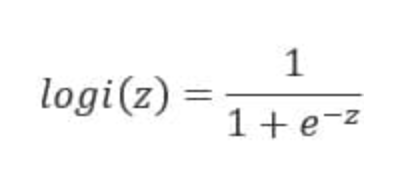
对应的函数图像可以表示如下:
import numpy as npimport matplotlib.pyplot as pltx = np.arange(-5,5,0.01)y = 1/(1+np.exp(-x))plt.plot(x,y)plt.xlabel('z')plt.ylabel('y')plt.grid()plt.show()
Output: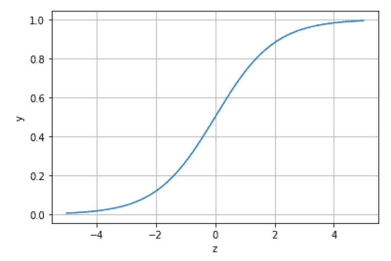
通过上图我们可以发现 Logistic 函数是单调递增函数,并且在z=0
而回归的基本方程,
将回归方程写入其中为: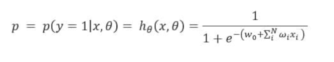
所以,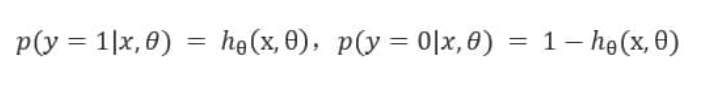
逻辑回归从其原理上来说,逻辑回归其实是实现了一个决策边界:对于函数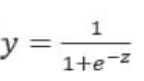 , 当z≥0 时,y≥0.5,分类为1,当 z<0时,y<0.5,分类为0,其对应的y值我们可以视为类别1的概率预测值。
对于模型的训练而言:实质上来说就是利用数据求解出对应的模型的特定的ω。从而得到一个针对于当前数据的特征逻辑回归模型。
而对于多分类而言,将多个二分类的逻辑回归组合,即可实现多分类。
= = = = = END FOR ALL TASK01 = = = = =

若有收获,就点个赞吧
0 人点赞
