8.1 循环神经网络

8.1 序列模型

8.1.1 序列模型的统计工具

表示时间，。序列模型就是在发生的情况下，预测：
%0A#card=math&code=x%7Bt%7D%20%5Csim%20P%5Cleft%28x%7Bt%7D%20%5Cmid%20x%7Bt-1%7D%2C%20%5Cldots%2C%20x%7B1%7D%5Cright%29%0A&id=l2IV7)
序列模型的估计需要专门的统计工具，两种较流行的选择是自回归模型和隐变量自回归模型。
第一种策略，使用满足某个长度为τ的时间跨度， 即使用观测序列。 当t>τ时参数的数量总是不变的。 这种模型被称为自回归模型（autoregressive models）。
第二种策略， 保留一些对过去观测的总结#card=math&code=h%7Bt%7D%3Df%28x%7B1%7D%2C%5Cdots%2Cx%7Bt-1%7D%29&id=quwVj)， 并且同时更新预测和总结。 这就产生了基于#card=math&code=%5Chat%7Bx%7D%7Bt%7D%3DP%5Cleft%28x%7Bt%7D%20%5Cmid%20h%7Bt%7D%5Cright%29&id=InAeE)估计， 以及公式#card=math&code=h%7Bt%7D%3Dg%28h%7Bt%E2%88%921%7D%2Cx%7Bt%E2%88%921%7D%29&id=FqYw9)更新的模型。 由于从未被观测到，这类模型被称为 隐变量自回归模型（latent autoregressive models）。

序列的数据可能随着时间变化， 但是序列本身的动力学不会改变。整个序列的估计值将通过以下的方式获得（条件概率展开）：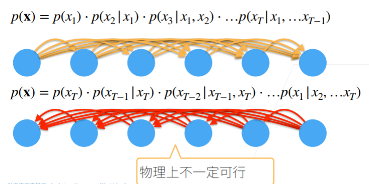

如果序列中的值 的值仅与有关，而与无关，就说序列满足马尔可夫性（Markov condition），也称无后效性。如果τ=1，得到 一阶马尔可夫模型（first-order Markov model）， P(x)由下式给出：
%3D%5Cprod%7Bt%3D1%7D%5E%7BT%7D%20P%5Cleft(x%7Bt%7D%20%5Cmid%20x%7Bt-1%7D%5Cright)%20%E5%BD%93P(x%7B1%7D%7Cx%7B0%7D)%3DP(x%7B1%7D)%0A#card=math&code=P%5Cleft%28x%7B1%7D%2C%20%5Cldots%2C%20x%7BT%7D%5Cright%29%3D%5Cprod%7Bt%3D1%7D%5E%7BT%7D%20P%5Cleft%28x%7Bt%7D%20%5Cmid%20x%7Bt-1%7D%5Cright%29%20%E5%BD%93P%28x%7B1%7D%7Cx%7B0%7D%29%3DP%28x_%7B1%7D%29%0A&id=oYIzE)
利用这一事实，我们只需考虑过去观察中一个非常短的历史。

8.1.2 训练

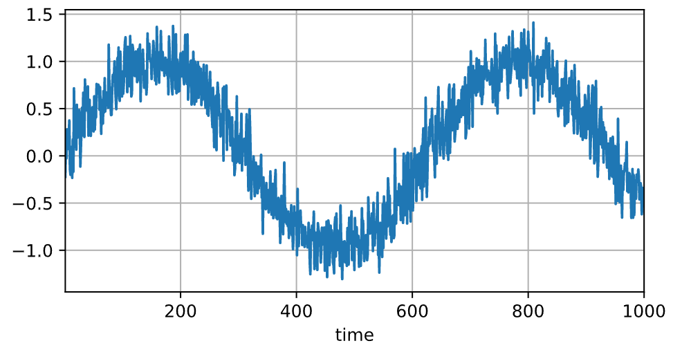
下面使用正弦函数和可加性噪声来生成序列数据。

import torch
from torch import nn
from d2l import torch as d2l
T = 1000  # 总共产生1000个点
time = torch.arange(1, T + 1, dtype=torch.float32)
x = torch.sin(0.01 * time) + torch.normal(0, 0.2, (T,))
d2l.plot(time, [x], 'time', 'x', xlim=[1, 1000], figsize=(6, 3))

# 基于嵌入维度tau，生成对应的特征-标签对
tau = 4
features = torch.zeros((T - tau, tau))# 每个特征包含4个属性，因此可生成T-tau个对象
for i in range(tau):
    features[:, i] = x[i: T - tau + i]# 从第一个开始生成
labels = x[tau:].reshape((-1, 1))# 从tau开始生成标签
batch_size, n_train = 16, 600
# 只有前n_train个样本用于训练
train_iter = d2l.load_array((features[:n_train], labels[:n_train]),
                            batch_size, is_train=True)
# 初始化网络权重的函数
def init_weights(m):
    if type(m) == nn.Linear:
        nn.init.xavier_uniform_(m.weight)
# 一个简单的多层感知机
def get_net():
    net = nn.Sequential(nn.Linear(4, 10),
                        nn.ReLU(),
                        nn.Linear(10, 1))
    net.apply(init_weights)
    return net
# 平方损失。注意：MSELoss计算平方误差时不带系数1/2
loss = nn.MSELoss(reduction='none')
def train(net, train_iter, loss, epochs, lr):
    trainer = torch.optim.Adam(net.parameters(), lr)
    for epoch in range(epochs):
        for X, y in train_iter:
            trainer.zero_grad()
            l = loss(net(X), y)
            l.sum().backward()
            trainer.step()
        print(f'epoch {epoch + 1}, '
              f'loss: {d2l.evaluate_loss(net, train_iter, loss):f}')
net = get_net()
train(net, train_iter, loss, 5, 0.01)
"""
epoch 1, loss: 0.081058
epoch 2, loss: 0.064629
epoch 3, loss: 0.058360
epoch 4, loss: 0.054131
epoch 5, loss: 0.052486
"""

8.1.3 预测

# 进行单步预测
onestep_preds = net(features)
d2l.plot([time, time[tau:]],
         [x.detach().numpy(), onestep_preds.detach().numpy()], 'time',
         'x', legend=['data', '1-step preds'], xlim=[1, 1000],
         figsize=(6, 3))

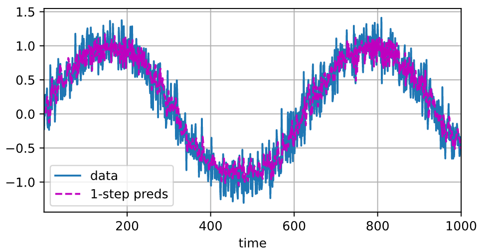
训练时仅使用了前600个“特征-标签”对进行训练，但是预测模型中，即使超出了600，预测效果依旧很棒。当然，这个数据是原先产生的，预测时并未采用预测生成的数据。如果使用预测时生成的数据，随着时间的推移，预测精度难免会逐步下降。例如，未来24小时的天气预报往往相当准确， 但超过这一点，精度就会迅速下降。

8.2 文本预处理

1. 将字符串拆分为词元（如单词和字符）。
2. 建立一个词表，将拆分的词元映射到数字索引。
3. 将文本转换为数字索引序列。

从H.G.Well的时光机器中加载文本。

#@save
d2l.DATA_HUB['time_machine'] = (d2l.DATA_URL + 'timemachine.txt',
                                '090b5e7e70c295757f55df93cb0a180b9691891a')
def read_time_machine():  #@save
    """将时间机器数据集加载到文本行的列表中"""
    with open(d2l.download('time_machine'), 'r') as f:
        lines = f.readlines()
    return [re.sub('[^A-Za-z]+', ' ', line).strip().lower() for line in lines]    # 忽略标点符号与字母大小写
lines = read_time_machine()

每个文本序列将被拆分成一个词元列表，词元（token）是文本的基本单位。 最后，返回一个由词元列表组成的列表，其中的每个词元都是一个字符串（string）。

def tokenize(lines, token='word'):  #@save
    """将文本行拆分为单词或字符词元，并返回由词元（token）列表组成的列表"""
    if token == 'word':
        return [line.split() for line in lines]
    elif token == 'char':
        return [list(line) for line in lines]    # 将字符串转化为字符列表
    else:
        print('错误：未知词元类型：' + token)
tokens = tokenize(lines)
"""
以词为单位的分词效果
['the', 'time', 'machine', 'by', 'h', 'g', 'wells']
"""

字典也叫做词表（vocabulary），用来将字符串类型的词元映射到从0开始的数字索引中。先将训练集中的唯一词元进行统计， 得到的结果称之为语料（corpus）。 然后根据每个唯一词元的出现频率，为其分配一个数字索引。 很少出现的词元通常被移除，可以降低复杂性。 另外，语料库中不存在或已删除的任何词元都将映射到一个特定的未知词元<unk>。 可以在参数中增加一个列表，用于保存那些被保留的词元， 例如：填充词元<pad>； 序列开始词元<bos>； 序列结束词元<eos>。

class Vocab:  #@save
    """文本词表"""
    def __init__(self, tokens=None, min_freq=0, reserved_tokens=None):
        if tokens is None:
            tokens = []
        if reserved_tokens is None:    # 预留词元
            reserved_tokens = []
        # 按出现频率排序
        counter = count_corpus(tokens)
        self._token_freqs = sorted(counter.items(), key=lambda x: x[1],
                                   reverse=True)
        # 未知词元的索引为0
        self.idx_to_token = ['<unk>'] + reserved_tokens
        self.token_to_idx = {token: idx
                             for idx, token in enumerate(self.idx_to_token)}
        for token, freq in self._token_freqs:    # 从高频到低频扩充词元
            if freq < min_freq:    # 频率低于最低频率就丢弃
                break
            if token not in self.token_to_idx:
                self.idx_to_token.append(token)
                self.token_to_idx[token] = len(self.idx_to_token) - 1
    def __len__(self):
        return len(self.idx_to_token)
    def __getitem__(self, tokens):
        if not isinstance(tokens, (list, tuple)):    # 单个词元
            return self.token_to_idx.get(tokens, self.unk)
        return [self.__getitem__(token) for token in tokens]    # 列表或元组
    def to_tokens(self, indices):
        if not isinstance(indices, (list, tuple)):
            return self.idx_to_token[indices]
        return [self.idx_to_token[index] for index in indices]
    @property
    def unk(self):  # 未知词元的索引为0
        return 0
    @property
    def token_freqs(self):
        return self._token_freqs
def count_corpus(tokens):  #@save
    """统计词元的频率"""
    # tokens为2D列表，每行为一句话的所有词元
    if len(tokens) == 0 or isinstance(tokens[0], list):
        # 将词元列表展平成一个列表
        tokens = [token for line in tokens for token in line]
    return collections.Counter(tokens)
# 使用时光机器数据集作为语料库构建词典
vocab = Vocab(tokens)
# 将每一条文本行转换成一个数字索引列表。
for i in [0, 10]:
    print('文本:', tokens[i])
    print('索引:', vocab[tokens[i]])
"""
文本: ['the', 'time', 'machine', 'by', 'h', 'g', 'wells']
索引: [1, 19, 50, 40, 2183, 2184, 400]
文本: ['twinkled', 'and', 'his', 'usually', 'pale', 'face', 'was', 'flushed', 'and', 'animated', 'the']
索引: [2186, 3, 25, 1044, 362, 113, 7, 1421, 3, 1045, 1]
"""

1. 为了简化后面章节中的训练，使用字符（而不是单词）实现文本词元化；
2. 时光机器数据集中的每个文本行不一定是一个句子或一个段落，还可能是一个单词，因此返回的corpus仅处理为单个列表，而不是使用多词元列表构成的一个列表。 ```python def load_corpus_time_machine(max_tokens=-1): #@save “””返回时光机器数据集的词元索引列表和词表””” lines = read_time_machine() tokens = tokenize(lines, ‘char’) vocab = Vocab(tokens) corpus = [vocab[token] for line in tokens for token in line] if max_tokens > 0:

    corpus = corpus[:max_tokens]

   return corpus, vocab

corpus, vocab = load_corpus_time_machine() len(corpus), len(vocab)# (170580, 28) # 以字符构建，因此词典为26个英文字母+空格+

<a name="0de4e0d3"></a>
## 8.3. 语言模型和数据集
语言模型（language model）的目标是估计序列的联合概率:<br />![](https://g.yuque.com/gr/latex?P(x_%7B1%7D%2Cx_%7B2%7D%2C%5Cdots%2Cx_%7BT%7D)%0A#card=math&code=P%28x_%7B1%7D%2Cx_%7B2%7D%2C%5Cdots%2Cx_%7BT%7D%29%0A&id=TrRhH)<br />一个理想的语言模型可以通过给定的初始词元，不断使用![](https://g.yuque.com/gr/latex?x_%7Bt%7D%5Csim%20P(x_%7Bt%7D%7Cx_%7Bt-1%7D%2C%5Cdots%2Cx_%7B1%7D)#card=math&code=x_%7Bt%7D%5Csim%20P%28x_%7Bt%7D%7Cx_%7Bt-1%7D%2C%5Cdots%2Cx_%7B1%7D%29&id=QSxEK)生成自然文本。显然离设计出这样的系统还很遥远， 因为它需要“理解”文本，而不仅仅是生成语法合理的内容。尽管如此，语言模型依然是非常有用的。 例如，短语“to recognize speech”和“to wreck a nice beach”读音上听起来非常相似。 这种相似性会导致语音识别中的歧义，但是这很容易通过语言模型来解决， 因为第二句的语义很奇怪。 同样，在文档摘要生成算法中， “狗咬人”比“人咬狗”出现的频率要高得多。
<a name="cd5b5930"></a>
### 8.3.1 学习语言模型
![](https://g.yuque.com/gr/latex?P(deep%2Clearning%2Cis%2Cfun)%3DP(deep)P(learning%E2%88%A3deep)%5C%5CP(is%E2%88%A3deep%2Clearning)P(fun%E2%88%A3deep%2Clearning%2Cis).%0A#card=math&code=P%28deep%2Clearning%2Cis%2Cfun%29%3DP%28deep%29P%28learning%E2%88%A3deep%29%5C%5CP%28is%E2%88%A3deep%2Clearning%29P%28fun%E2%88%A3deep%2Clearning%2Cis%29.%0A&id=mQ5z5)<br />为了训练语言模型，需要计算单词的概率， 以及给定前面几个单词后出现某个单词的条件概率。词的概率可以根据给定词的相对词频来计算。对于词deep，一种（稍稍不太精确的）方法是统计单词“deep”在数据集中的出现次数， 然后将其除以整个语料库中的单词总数。 这种方法效果不错，特别是对于频繁出现的单词。接下来可以尝试估计：<br />![](https://g.yuque.com/gr/latex?%5Chat%7BP%7D(learning%7Cdeep)%3D%5Cfrac%7Bn(deep%2Clearning)%7D%7Bn(deep)%7D%0A#card=math&code=%5Chat%7BP%7D%28learning%7Cdeep%29%3D%5Cfrac%7Bn%28deep%2Clearning%29%7D%7Bn%28deep%29%7D%0A&id=ABybB)<br />不幸的是，由于连续单词对“deep learning”的出现频率要低得多， 所以估计这类单词正确的概率要困难得多。 许多合理的三个单词组合可能是存在的，但是在数据集中却找不到。 除非我们提供某种解决方案，来将这些单词组合指定为非零计数， 否则将无法在语言模型中使用它们。<br />然而，这样的模型很容易变得无效，原因如下： 首先，我们需要存储所有的计数； 其次，这完全忽略了单词的意思。例如，“猫”（cat）和“猫科动物”（feline）可能出现在相关的上下文中， 但是想根据上下文调整这类模型其实是相当困难的。 最后，长单词序列大部分是没出现过的， 因此一个模型如果只是简单地统计先前“看到”的单词序列频率， 那么模型面对这种问题肯定是表现不佳的。
<a name="94ea1b42"></a>
### 8.3.2. 马尔可夫模型与n元语法
如果![](https://g.yuque.com/gr/latex?P(x_%7Bt%2B1%7D%E2%88%A3x_%7Bt%7D%2C%5Cdots%2Cx_%7B1%7D)%3DP(x_%7Bt%2B1%7D%E2%88%A3x_%7Bt%7D)#card=math&code=P%28x_%7Bt%2B1%7D%E2%88%A3x_%7Bt%7D%2C%5Cdots%2Cx_%7B1%7D%29%3DP%28x_%7Bt%2B1%7D%E2%88%A3x_%7Bt%7D%29&id=noUlF)，则序列上的分布满足一阶马尔可夫性。阶数越高，对应的依赖关系就越长。 这种性质推导出了许多可以应用于序列建模的近似公式：<br />![](https://g.yuque.com/gr/latex?%5Cbegin%7Barray%7D%7Bl%7D%0AP%5Cleft(x_%7B1%7D%2C%20x_%7B2%7D%2C%20x_%7B3%7D%2C%20x_%7B4%7D%5Cright)%3DP%5Cleft(x_%7B1%7D%5Cright)%20P%5Cleft(x_%7B2%7D%5Cright)%20P%5Cleft(x_%7B3%7D%5Cright)%20P%5Cleft(x_%7B4%7D%5Cright)%20%5C%5C%0AP%5Cleft(x_%7B1%7D%2C%20x_%7B2%7D%2C%20x_%7B3%7D%2C%20x_%7B4%7D%5Cright)%3DP%5Cleft(x_%7B1%7D%5Cright)%20P%5Cleft(x_%7B2%7D%20%5Cmid%20x_%7B1%7D%5Cright)%20P%5Cleft(x_%7B3%7D%20%5Cmid%20x_%7B2%7D%5Cright)%20P%5Cleft(x_%7B4%7D%20%5Cmid%20x_%7B3%7D%5Cright)%20%5C%5C%0AP%5Cleft(x_%7B1%7D%2C%20x_%7B2%7D%2C%20x_%7B3%7D%2C%20x_%7B4%7D%5Cright)%3DP%5Cleft(x_%7B1%7D%5Cright)%20P%5Cleft(x_%7B2%7D%20%5Cmid%20x_%7B1%7D%5Cright)%20P%5Cleft(x_%7B3%7D%20%5Cmid%20x_%7B1%7D%2C%20x_%7B2%7D%5Cright)%20P%5Cleft(x_%7B4%7D%20%5Cmid%20x_%7B2%7D%2C%20x_%7B3%7D%5Cright)%0A%5Cend%7Barray%7D%0A#card=math&code=%5Cbegin%7Barray%7D%7Bl%7D%0AP%5Cleft%28x_%7B1%7D%2C%20x_%7B2%7D%2C%20x_%7B3%7D%2C%20x_%7B4%7D%5Cright%29%3DP%5Cleft%28x_%7B1%7D%5Cright%29%20P%5Cleft%28x_%7B2%7D%5Cright%29%20P%5Cleft%28x_%7B3%7D%5Cright%29%20P%5Cleft%28x_%7B4%7D%5Cright%29%20%5C%5C%0AP%5Cleft%28x_%7B1%7D%2C%20x_%7B2%7D%2C%20x_%7B3%7D%2C%20x_%7B4%7D%5Cright%29%3DP%5Cleft%28x_%7B1%7D%5Cright%29%20P%5Cleft%28x_%7B2%7D%20%5Cmid%20x_%7B1%7D%5Cright%29%20P%5Cleft%28x_%7B3%7D%20%5Cmid%20x_%7B2%7D%5Cright%29%20P%5Cleft%28x_%7B4%7D%20%5Cmid%20x_%7B3%7D%5Cright%29%20%5C%5C%0AP%5Cleft%28x_%7B1%7D%2C%20x_%7B2%7D%2C%20x_%7B3%7D%2C%20x_%7B4%7D%5Cright%29%3DP%5Cleft%28x_%7B1%7D%5Cright%29%20P%5Cleft%28x_%7B2%7D%20%5Cmid%20x_%7B1%7D%5Cright%29%20P%5Cleft%28x_%7B3%7D%20%5Cmid%20x_%7B1%7D%2C%20x_%7B2%7D%5Cright%29%20P%5Cleft%28x_%7B4%7D%20%5Cmid%20x_%7B2%7D%2C%20x_%7B3%7D%5Cright%29%0A%5Cend%7Barray%7D%0A&id=DfTxJ)<br />通常，涉及一个、两个和三个变量的概率公式分别被称为 “一元语法”（unigram）、“二元语法”（bigram）和“三元语法”（trigram）模型。
<a name="00a20935"></a>
### 8.3.3. 自然语言统计
```python
# 一元语法词频统计
import random
import torch
from d2l import torch as d2l

tokens = d2l.tokenize(d2l.read_time_machine())
# 将每个句子的单词拼接到一个列表中
corpus = [token for line in tokens for token in line]
vocab = d2l.Vocab(corpus)    # 字典化
vocab.token_freqs[:10]    # 打印出现频率最高的前十个词
"""
[('the', 2261),
 ('i', 1267),
 ('and', 1245),
 ('of', 1155),
 ('a', 816),
 ('to', 695),
 ('was', 552),
 ('in', 541),
 ('that', 443),
 ('my', 440)]
"""

部分没有实际意义的词通常被称为停用词（stop words），可以过滤掉以降低模型复杂度。还有个明显的问题是词频衰减的速度相当地快。

# 二元语法词频统计
bigram_tokens = [pair for pair in zip(corpus[:-1], corpus[1:])]
bigram_vocab = d2l.Vocab(bigram_tokens)
bigram_vocab.token_freqs[:10]
"""
[(('of', 'the'), 309),
 (('in', 'the'), 169),
 (('i', 'had'), 130),
 (('i', 'was'), 112),
 (('and', 'the'), 109),
 (('the', 'time'), 102),
 (('it', 'was'), 99),
 (('to', 'the'), 85),
 (('as', 'i'), 78),
 (('of', 'a'), 73)]
"""

在十个最频繁的词对中，有九个是由两个停用词组成的。

# 三元语法词频统计
trigram_tokens = [triple for triple in zip(
    corpus[:-2], corpus[1:-1], corpus[2:])]
trigram_vocab = d2l.Vocab(trigram_tokens)
trigram_vocab.token_freqs[:10]
"""
[(('the', 'time', 'traveller'), 59),
 (('the', 'time', 'machine'), 30),
 (('the', 'medical', 'man'), 24),
 (('it', 'seemed', 'to'), 16),
 (('it', 'was', 'a'), 15),
 (('here', 'and', 'there'), 15),
 (('seemed', 'to', 'me'), 14),
 (('i', 'did', 'not'), 14),
 (('i', 'saw', 'the'), 13),
 (('i', 'began', 'to'), 13)]
"""

最后，我们直观地对比三种模型中的词元频率：一元语法、二元语法和三元语法。

bigram_freqs = [freq for token, freq in bigram_vocab.token_freqs]
trigram_freqs = [freq for token, freq in trigram_vocab.token_freqs]
d2l.plot([freqs, bigram_freqs, trigram_freqs], xlabel='token: x',
         ylabel='frequency: n(x)', xscale='log', yscale='log',
         legend=['unigram', 'bigram', 'trigram'])

以一元词为例，将前几个词删除后，剩余单词大致遵循双对数坐标图[^1]上的一条直线。 这意味着单词的频率满足齐普夫定律（Zipf’s law）， 即第个最常用单词的频率为：

等价于

其中α是刻画分布的指数，c是常数。 在一元和二元模型中，想要通过计数统计和平滑来建模单词是不可行的， 因为这样建模的结果会大大高估不常用单词的频率。
一元、二元、三元单词序列似乎都遵循齐普夫定律，尽管α （受序列长度的影响）更小。其次，词表中n元组的数量并没有那么大， 给了我们应用模型的希望。 第三，很多n元组很少出现，这使得拉普拉斯平滑非常不适合语言建模。 作为代替，我们将使用基于深度学习的模型。

8.3.4. 读取长序列数据

模型中的网络一次仅可处理固定长度 （n个时间步）的小批量序列。 在8.1节的示例中，每一次的特征-标签对都通过移动一个步长来获得，每一个元素将被使用次，这使得每一个epoch处理的时间过长。为了解决这个问题，使用以固定步长切分句子的方式，这样每个epoch每个元素仅使用了一次。下图展示了当n=5，词元为一个字符的所有划分情况。

上面5种划分策略一样好， 如果只选择一个偏移量（上面有5种偏移量，分别为0,1,2,3,4），每个epoch都将使用相同的特征-标签对，而一部分特征-标签对不会被使用。因此可以从随机偏移量开始划分序列，保证所有的特征-标签对都覆盖。此外，为了防止模型记住输入序列的顺序关系，让模型有更好的泛化性，每次对所有切割后的序列进行随机抽取。下面将描述如何实现这种策略：
在随机采样中，每个样本都是在原始的长序列上任意捕获的子序列。 在迭代过程中，两个相邻的子序列不一定在原始序列上相邻。下面的代码参数batch_size指定了每个小批量中子序列样本的数目， 参数num_steps是每个子序列中预定义的时间步数。

def seq_data_iter_random(corpus, batch_size, num_steps):  #@save
    """使用随机抽样生成一个小批量子序列"""
    # 从随机偏移量开始对序列进行分区，随机范围包括num_steps-1
    corpus = corpus[random.randint(0, num_steps - 1):]
    # 减去1，是因为我们需要考虑标签
    num_subseqs = (len(corpus) - 1) // num_steps
    # 长度为num_steps的子序列的起始索引
    initial_indices = list(range(0, num_subseqs * num_steps, num_steps))
    # 在随机抽样的迭代过程中，
    # 来自两个相邻的、随机的、小批量中的子序列不一定在原始序列上相邻
    random.shuffle(initial_indices)

    def data(pos):
        # 返回从pos位置开始的长度为num_steps的序列
        return corpus[pos: pos + num_steps]

    num_batches = num_subseqs // batch_size
    for i in range(0, batch_size * num_batches, batch_size):
        # 在这里，initial_indices包含子序列的随机起始索引
        initial_indices_per_batch = initial_indices[i: i + batch_size]
        X = [data(j) for j in initial_indices_per_batch]
        Y = [data(j + 1) for j in initial_indices_per_batch]
        yield torch.tensor(X), torch.tensor(Y)

下面生成一个从0到34的序列。 假设批量大小为2，时间步数为5，这意味着可以生成 ⌊(35−1)/5⌋=6个“特征－标签”子序列对。 如果设置小批量大小为2，我们只能得到3个小批量。

my_seq = list(range(35))
for X, Y in seq_data_iter_random(my_seq, batch_size=2, num_steps=5):
    print('X: ', X, '\nY:', Y)
"""
X:  tensor([[29, 30, 31, 32, 33],
        [ 4,  5,  6,  7,  8]])
Y: tensor([[30, 31, 32, 33, 34],
        [ 5,  6,  7,  8,  9]])
X:  tensor([[ 9, 10, 11, 12, 13],
        [14, 15, 16, 17, 18]])
Y: tensor([[10, 11, 12, 13, 14],
        [15, 16, 17, 18, 19]])
X:  tensor([[24, 25, 26, 27, 28],
        [19, 20, 21, 22, 23]])
Y: tensor([[25, 26, 27, 28, 29],
        [20, 21, 22, 23, 24]])
"""

除了对原始序列随机抽样外， 还有另一种策略保证两个相邻的小批量中的子序列在原始序列上也是相邻的。 这种策略被称为顺序分区。

def seq_data_iter_sequential(corpus, batch_size, num_steps):  #@save
    """使用顺序分区生成一个小批量子序列"""
    # 从随机偏移量开始划分序列
    offset = random.randint(0, num_steps)
    # 保证每个batch有相同token数时，共可利用的token数
    num_tokens = ((len(corpus) - offset - 1) // batch_size) * batch_size
    Xs = torch.tensor(corpus[offset: offset + num_tokens])
    Ys = torch.tensor(corpus[offset + 1: offset + 1 + num_tokens])
    Xs, Ys = Xs.reshape(batch_size, -1), Ys.reshape(batch_size, -1)
    num_batches = Xs.shape[1] // num_steps    #  
    for i in range(0, num_steps * num_batches, num_steps):
        X = Xs[:, i: i + num_steps]
        Y = Ys[:, i: i + num_steps]
        yield X, Y

# 获取顺序分区的小批量子序列
for X, Y in seq_data_iter_sequential(my_seq, batch_size=2, num_steps=5):
    print('X: ', X, '\nY:', Y)
"""
X:  tensor([[ 3,  4,  5,  6,  7],
        [18, 19, 20, 21, 22]])
Y: tensor([[ 4,  5,  6,  7,  8],
        [19, 20, 21, 22, 23]])
X:  tensor([[ 8,  9, 10, 11, 12],
        [23, 24, 25, 26, 27]])
Y: tensor([[ 9, 10, 11, 12, 13],
        [24, 25, 26, 27, 28]])
X:  tensor([[13, 14, 15, 16, 17],
        [28, 29, 30, 31, 32]])
Y: tensor([[14, 15, 16, 17, 18],
        [29, 30, 31, 32, 33]])
"""

将上面的两个采样函数包装到一个类中， 以便稍后可以将其用作数据迭代器。

class SeqDataLoader:  #@save
    """加载序列数据的迭代器"""
    def __init__(self, batch_size, num_steps, use_random_iter, max_tokens):
        if use_random_iter:    # 使用随机迭代器
            self.data_iter_fn = d2l.seq_data_iter_random
        else:    # 使用顺序迭代器
            self.data_iter_fn = d2l.seq_data_iter_sequential
        self.corpus, self.vocab = d2l.load_corpus_time_machine(max_tokens)
        self.batch_size, self.num_steps = batch_size, num_steps

    def __iter__(self):
        return self.data_iter_fn(self.corpus, self.batch_size, self.num_steps)

最后定义函数load_data_time_machine， 它同时返回数据迭代器和词表， 因此可以与其他带有load_data前缀的函数 （如 3.5节中定义的 d2l.load_data_fashion_mnist）类似地使用。

def load_data_time_machine(batch_size, num_steps,  #@save
                           use_random_iter=False, max_tokens=10000):
    """返回时光机器数据集的迭代器和词表"""
    data_iter = SeqDataLoader(
        batch_size, num_steps, use_random_iter, max_tokens)
    return data_iter, data_iter.vocab

8.4. 循环神经网络

元语法模型中单词在时间步的条件概率取决于前面个单词，即将#card=math&code=P%28x%7Bt%7D%E2%88%A3x%7Bt%E2%88%921%7D%2C%E2%80%A6%2Cx%7Bt%E2%88%92n%2B1%7D%29&id=L0n39)模型化。然而模型参数的数量也会随之呈指数增长， 因为词表需要存储个数字，这不如使用隐变量模型：
%20%5Capprox%20P%5Cleft(x%7Bt%7D%20%5Cmid%20h%7Bt-1%7D%5Cright)%0A#card=math&code=P%5Cleft%28x%7Bt%7D%20%5Cmid%20x%7Bt-1%7D%2C%20%5Cldots%2C%20x%7B1%7D%5Cright%29%20%5Capprox%20P%5Cleft%28x%7Bt%7D%20%5Cmid%20h%7Bt-1%7D%5Cright%29%0A&id=TZau2)
其中是隐状态（hidden state），也称为隐藏变量（hidden variable）， 它存储了序列直到时间步的序列信息，相当于当前情况下，神经网络的状态或记忆。可以基于当前输入和先前隐状态 来计算时间步处的隐状态：
%0A#card=math&code=h%7Bt%7D%3Df%28x%7Bt%7D%2Ch_%7Bt-1%7D%29%0A&id=PAhq5)
循环神经网络（recurrent neural networks，RNNs） 是具有隐状态的神经网络。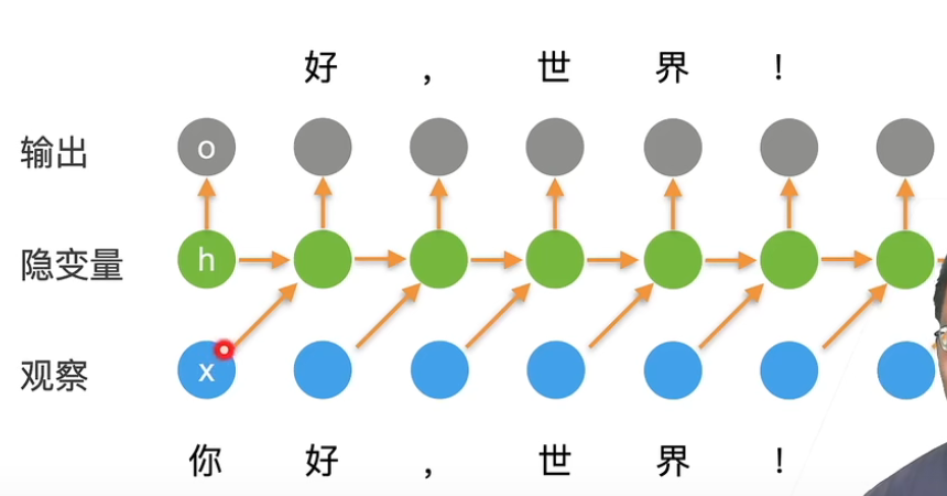

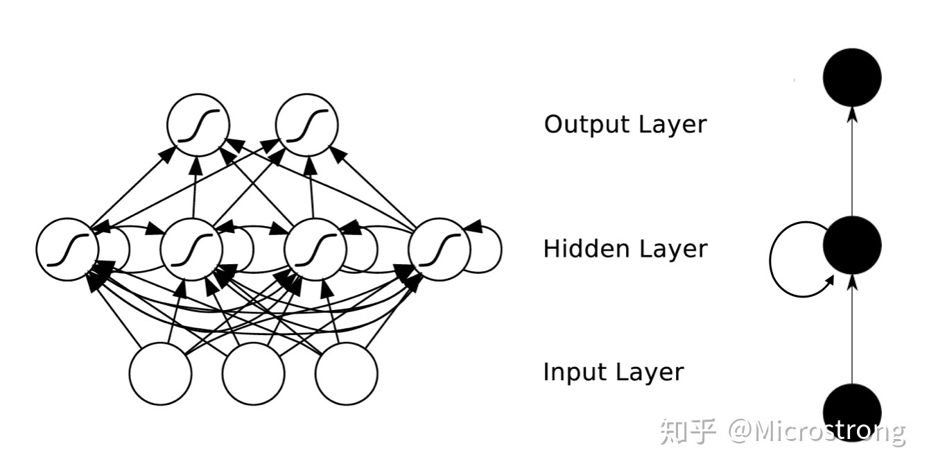
8.4.1. 有隐状态的神经网络

假设在时间步有小批量输入，用表示时间步的隐藏变量，新的权重参数描述如何在当前时间步中使用前一个时间步的隐藏变量。
%0A#card=math&code=%5Cmathbf%7BH%7D%7Bt%7D%3D%CF%95%28%5Cmathbf%7BX%7D%7Bt%7D%5Cmathbf%7BW%7D%7Bxh%7D%2B%5Cmathbf%7BH%7D%7Bt-1%7D%5Cmathbf%7BW%7D%7Bhh%7D%2B%5Cmathbf%7Bb%7D%7Bh%7D%29%0A&id=HS9S0)
由于在当前时间步中， 隐状态使用的定义与前一个时间步中使用的定义相同，因此上式的计算是循环的（recurrent）。于是基于循环计算的隐状态神经网络被命名为 循环神经网络（recurrent neural network）。 在循环神经网络中执行上述计算的层 称为循环层（recurrent layer）。

即使在不同的时间步，循环神经网络也总是使用这些模型参数。因此，循环神经网络的参数开销不会随着时间步的增加而增加。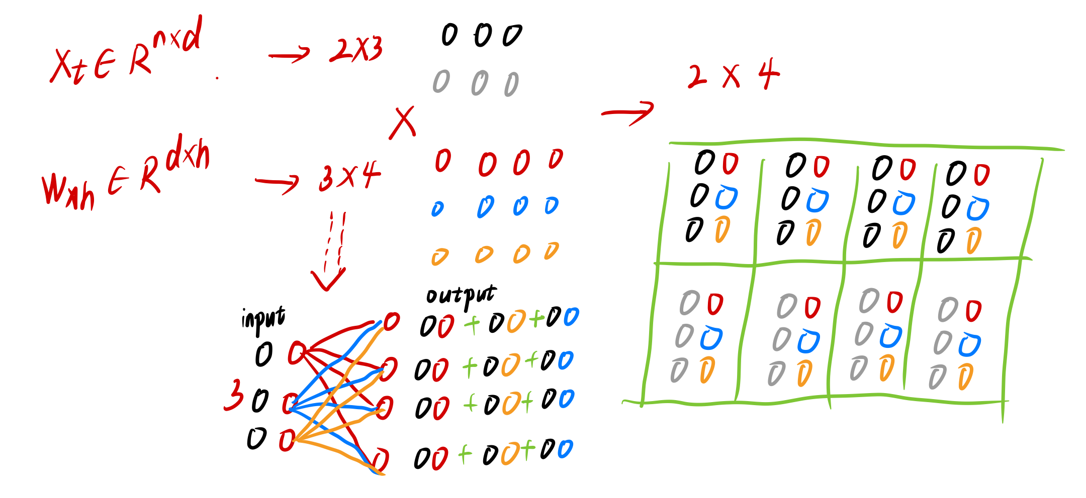


RNN内部计算时，隐状态中的计算会转化为和的拼接与和的拼接的矩阵乘法。定义矩阵X、W_xh、H和W_hh， 它们的形状分别为(3，1)、(1，4)、(3，4)和(4，4)，按计算后结果形状为(3, 4)。在拼接时，和按列拼接，拼接后的形状为(3,5)，和按行拼接，拼接后为(5,4)，两者的矩阵乘法(torch.matmul())为(3,4)且结果相同（矩阵分块原理）。拼接后的张量将通过一个全连接层，最终得到该时间步的输出与结果。

8.4.2. 困惑度（Perplexity）

语言生成问题可以等价为分类问题，因此可以使用交叉熵作为损失函数。设集合中包含n个词语，等价于是一个n分类问题，因此可以通过n个词元的交叉熵损失的平均值来度量语言模型的质量：
%0A#card=math&code=%5Cfrac%7B1%7D%7Bn%7D%20%5Csum%7Bt%3D1%7D%5E%7Bn%7D-%5Clog%20P%5Cleft%28x%7Bt%7D%20%5Cmid%20x%7Bt-1%7D%2C%20%5Cldots%2C%20x%7B1%7D%5Cright%29%0A&id=mpI4j)
困惑度（perplexity）是上式的指数：
)%0A#card=math&code=exp%28-%5Cfrac%7B1%7D%7Bn%7D%20%5Csum%7Bt%3D1%7D%5E%7Bn%7D-%5Clog%20P%5Cleft%28x%7Bt%7D%20%5Cmid%20x%7Bt-1%7D%2C%20%5Cldots%2C%20x%7B1%7D%5Cright%29%29%0A&id=vhgND)

• 在最好的情况下，模型总是完美地估计标签词元的概率为1。 在这种情况下，模型的困惑度为1。
• 在最坏的情况下，模型总是预测标签词元的概率为0。 在这种情况下，困惑度是正无穷大。

  8.4.3 RNN的分类

  按照输入和输出的结构进行分类
  

  8.5. 循环神经网络的从零开始实现

  8.5.1 循环神经网络从零实现

  ```python import math import torch from torch import nn from torch.nn import functional as F from d2l import torch as d2l

读取数据集

batch_size, num_steps = 32, 35 train_iter, vocab = d2l.load_data_time_machine(batch_size, num_steps)

我们通常将每个词元表示为更具表现力的**特征向量**。最简单的表示称为**独热码**（one-hot encoding）。我们每次采样的小批量数据形状是二维张量： （批量大小，时间步数）。one_hot函数将这样一个小批量数据转换成三维张量，**张量的最后一个维度等于词表大小（len(vocab)）**。**我们经常转换输入的维度，以便获得形状为（时间步数，批量大小，词表大小）的输出。这将使我们能够更方便地通过最外层的维度，一步一步地更新小批量数据的隐状态。**时间步数对应![](https://g.yuque.com/gr/latex?t#card=math&code=t&id=Dk227)，批量大小对应![](https://g.yuque.com/gr/latex?n#card=math&code=n&id=r4nHb)，词表大小对应![](https://g.yuque.com/gr/latex?d#card=math&code=d&id=VOxSH)。
```python
X = torch.arange(10).reshape((2, 5))
F.one_hot(X.T, 28).shape    # torch.Size([5, 2, 28])

隐藏单元数num_hiddens是一个可调的超参数。当训练语言模型时，输入和输出来自相同的词表。因此，它们具有相同的维度，即词表的大小。

# 初始化模型参数
def get_params(vocab_size, num_hiddens, device):
    num_inputs = num_outputs = vocab_size

    def normal(shape):
        return torch.randn(size=shape, device=device) * 0.01

    # 隐藏层参数
    W_xh = normal((num_inputs, num_hiddens))
    W_hh = normal((num_hiddens, num_hiddens))
    b_h = torch.zeros(num_hiddens, device=device)
    # 输出层参数
    W_hq = normal((num_hiddens, num_outputs))
    b_q = torch.zeros(num_outputs, device=device)
    # 附加梯度
    params = [W_xh, W_hh, b_h, W_hq, b_q]
    for param in params:
        param.requires_grad_(True)
    return params

首先需要一个init_rnn_state函数在初始化时返回隐状态。 循环神经网络模型通过inputs最外层的维度实现循环， 以便逐时间步更新小批量数据的隐状态H。 此外，这里使用tanh函数作为激活函数。 如 4.1节所述， 当元素在实数上满足均匀分布时，tanh函数的平均值为0。

def init_rnn_state(batch_size, num_hiddens, device):
    # 可能存在多个隐藏层，为了后续方便处理，使用元组
    return (torch.zeros((batch_size, num_hiddens), device=device), )

# 在一个时间步内计算隐状态和输出
def rnn(inputs, state, params):
    # inputs的形状：(时间步数量，批量大小，词表大小)
    W_xh, W_hh, b_h, W_hq, b_q = params
    H, = state
    outputs = []
    # X的形状：(批量大小，词表大小)
    for X in inputs:    # 每次运行走完所有时间步
        H = torch.tanh(torch.mm(X, W_xh) + torch.mm(H, W_hh) + b_h)
        Y = torch.mm(H, W_hq) + b_q
        outputs.append(Y)
    return torch.cat(outputs, dim=0), (H,)

class RNNModelScratch: #@save
    """从零开始实现的循环神经网络模型"""
    def __init__(self, vocab_size, num_hiddens, device,
                 get_params, init_state, forward_fn):
        self.vocab_size, self.num_hiddens = vocab_size, num_hiddens
        self.params = get_params(vocab_size, num_hiddens, device)
        self.init_state, self.forward_fn = init_state, forward_fn

    def __call__(self, X, state):
        X = F.one_hot(X.T, self.vocab_size).type(torch.float32)
        return self.forward_fn(X, state, self.params)

    def begin_state(self, batch_size, device):
        return self.init_state(batch_size, self.num_hiddens, device)

num_hiddens = 512
net = RNNModelScratch(len(vocab), num_hiddens, d2l.try_gpu(), get_params,init_rnn_state, rnn)
state = net.begin_state(X.shape[0], d2l.try_gpu())
Y, new_state = net(X.to(d2l.try_gpu()), state)
Y.shape, len(new_state), new_state[0].shape

我们可以看到输出形状是（时间步数×批量大小，词表大小）， 而隐状态形状保持不变，即（批量大小，隐藏单元数）。

8.5.2 预测

在循环遍历prefix中的开始字符时不断地将隐状态传递到下一个时间步，但是不生成任何输出。 这被称为预热（warm-up）期， 因为在此期间模型会自我更新（例如，更新隐状态）， 但不会进行预测。 预热期结束后，隐状态的值通常比刚开始的初始值更适合预测， 从而预测字符并输出它们。隐状态在每次预测时都要重新初始化，因为其主要的作用是记录序列信息。

def predict_ch8(prefix, num_preds, net, vocab, device):  #@save
    """在prefix后面生成新字符"""
    state = net.begin_state(batch_size=1, device=device) # 初始化一个batch的隐状态
    outputs = [vocab[prefix[0]]]
    get_input = lambda: torch.tensor([outputs[-1]], device=device).reshape((1, 1))
    for y in prefix[1:]:  # 预热期。通过输入数据更新隐状态
        _, state = net(get_input(), state) # 获得新的隐状态state和输出_
        outputs.append(vocab[y])
    for _ in range(num_preds):  # 预测num_preds步
        y, state = net(get_input(), state)
        outputs.append(int(y.argmax(dim=1).reshape(1)))
    return ''.join([vocab.idx_to_token[i] for i in outputs])

predict_ch8('time traveller ', 10, net, vocab, d2l.try_gpu())
'time traveller a a a a a '

8.5.3. 梯度裁剪

在迭代中计算个时间步上的梯度，将会在反向传播中产生长度为#card=math&code=O%28T%29&id=vXABo)的矩阵乘法链。如 4.8节所述，当较大时可能导致梯度爆炸或梯度消失。
梯度爆炸可以通过降低学习率来解决。但如果很少得到大的梯度呢，这种做法就似乎毫无道理。一个流行的替代方案是通过将梯度投影回给定半径（例如）的球来裁剪梯度。如下式：
%20%5Cmathbf%7Bg%7D%0A#card=math&code=%5Cmathbf%7Bg%7D%20%5Cleftarrow%20%5Cmin%20%5Cleft%281%2C%20%5Cfrac%7B%5Ctheta%7D%7B%5C%7C%5Cmathbf%7Bg%7D%5C%7C%7D%5Cright%29%20%5Cmathbf%7Bg%7D%0A&id=dbMXq)
通过这样做，梯度范数永远不会超过。下面定义一个函数来裁剪模型的梯度：

def grad_clipping(net, theta):  #@save
    """裁剪梯度"""
    if isinstance(net, nn.Module):
        params = [p for p in net.parameters() if p.requires_grad]
    else:
        params = net.params
    norm = torch.sqrt(sum(torch.sum((p.grad ** 2)) for p in params))
    if norm > theta:
        for param in params:
            param.grad[:] *= theta / norm

8.5.4. 训练

1. 序列数据的不同采样方法（随机采样和顺序分区）将导致隐状态初始化的差异。
2. 更新模型参数之前裁剪梯度来缓解梯度爆照问题。
3. 用困惑度来评价模型， 确保了不同长度的序列具有可比性。

当使用顺序分区时，我们只在每个迭代周期的开始位置初始化隐状态。由于下一个小批量数据中的第i个子序列样本与当前第i个子序列样本相邻，因此当前小批量数据最后一个样本的隐状态，将用于初始化下一个小批量数据第一个样本的隐状态。这样，存储在隐状态中的序列的历史信息可以在一个迭代周期内流经相邻的子序列。
然而，在任何一点隐状态的计算，都依赖于同一迭代周期中前面所有的小批量数据， 这使得梯度计算变得复杂。为了降低计算量，在处理任何一个小批量数据之前，我们先分离梯度，使得隐状态的梯度计算总是限制在一个小批量数据的时间步内。当使用随机抽样时，因为每个样本都是在一个随机位置抽样的，因此需要为每个迭代周期重新初始化隐状态。

#@save
def train_epoch_ch8(net, train_iter, loss, updater, device, use_random_iter):
    """训练网络一个迭代周期（定义见第8章）"""
    state, timer = None, d2l.Timer()
    metric = d2l.Accumulator(2)  # 训练损失之和,词元数量
    for X, Y in train_iter:
        if state is None or use_random_iter:
            # 在第一次迭代或使用随机抽样时初始化state
            state = net.begin_state(batch_size=X.shape[0], device=device)
        else:
            if isinstance(net, nn.Module) and not isinstance(state, tuple):
                # state对于nn.GRU是个张量
                state.detach_()
            else:
                # state对于nn.LSTM或对于我们从零开始实现的模型是个张量
                for s in state:
                    s.detach_()
        y = Y.T.reshape(-1)
        X, y = X.to(device), y.to(device)
        y_hat, state = net(X, state)
        l = loss(y_hat, y.long()).mean()
        if isinstance(updater, torch.optim.Optimizer):
            updater.zero_grad()
            l.backward()
            grad_clipping(net, 1)
            updater.step()
        else:
            l.backward()
            grad_clipping(net, 1)
            # 因为已经调用了mean函数
            updater(batch_size=1)
        metric.add(l * y.numel(), y.numel())
    return math.exp(metric[0] / metric[1]), metric[1] / timer.stop()

循环神经网络模型的训练函数既支持从零开始实现， 也可以使用高级API来实现。

#@save
def train_ch8(net, train_iter, vocab, lr, num_epochs, device,
              use_random_iter=False):
    """训练模型（定义见第8章）"""
    loss = nn.CrossEntropyLoss()
    animator = d2l.Animator(xlabel='epoch', ylabel='perplexity',
                            legend=['train'], xlim=[10, num_epochs])
    # 初始化
    if isinstance(net, nn.Module):
        updater = torch.optim.SGD(net.parameters(), lr)
    else:
        updater = lambda batch_size: d2l.sgd(net.params, lr, batch_size)
    predict = lambda prefix: predict_ch8(prefix, 50, net, vocab, device)
    # 训练和预测
    for epoch in range(num_epochs):
        ppl, speed = train_epoch_ch8(
            net, train_iter, loss, updater, device, use_random_iter)
        if (epoch + 1) % 10 == 0:
            print(predict('time traveller'))
            animator.add(epoch + 1, [ppl])
    print(f'困惑度 {ppl:.1f}, {speed:.1f} 词元/秒 {str(device)}')
    print(predict('time traveller'))
    print(predict('traveller'))

因为数据集中使用了10000个词元，所以模型需要更多的迭代周期来更好地收敛。

num_epochs, lr = 500, 1
train_ch8(net, train_iter, vocab, lr, num_epochs, d2l.try_gpu())

最后，让我们检查一下使用随机抽样方法的结果。

net = RNNModelScratch(len(vocab), num_hiddens, d2l.try_gpu(), get_params,
                      init_rnn_state, rnn)
train_ch8(net, train_iter, vocab, lr, num_epochs, d2l.try_gpu(),
          use_random_iter=True)

8.6. 循环神经网络的简洁实现

import torch
from torch import nn
from torch.nn import functional as F
from d2l import torch as d2l

# 获取数据
batch_size, num_steps = 32, 35
train_iter, vocab = d2l.load_data_time_machine(batch_size, num_steps)
# 构造一个具有256个隐藏单元的单隐藏层的循环神经网络层rnn_layer。
num_hiddens = 256
rnn_layer = nn.RNN(len(vocab), num_hiddens)    # 输入维度d为one-hot长度，即词表长度
# 使用张量来初始化隐状态，它的形状是（隐藏层数，批量大小，隐藏单元数）
state = torch.zeros((1, batch_size, num_hiddens))
state.shape    # torch.Size([1, 32, 256])
# rnn_layer的“输出”（Y）不涉及输出层的计算：它是指每个时间步的隐状态，这些隐状态可以用作后续输出层的输入
X = torch.rand(size=(num_steps, batch_size, len(vocab)))
Y, state_new = rnn_layer(X, state)
Y.shape, state_new.shape    # (torch.Size([35, 32, 256]), torch.Size([1, 32, 256]))

#@save
class RNNModel(nn.Module):
    """循环神经网络模型"""
    def __init__(self, rnn_layer, vocab_size, **kwargs):
        super(RNNModel, self).__init__(**kwargs)
        self.rnn = rnn_layer
        self.vocab_size = vocab_size
        self.num_hiddens = self.rnn.hidden_size
        # 创建单独输出层：如果RNN是双向的（之后将介绍），num_directions应该是2，否则应该是1。
        if not self.rnn.bidirectional:
            self.num_directions = 1
            self.linear = nn.Linear(self.num_hiddens, self.vocab_size)
        else:
            self.num_directions = 2
            self.linear = nn.Linear(self.num_hiddens * 2, self.vocab_size)

    def forward(self, inputs, state):
        X = F.one_hot(inputs.T.long(), self.vocab_size)
        X = X.to(torch.float32)
        Y, state = self.rnn(X, state)
        # 全连接层首先将Y的形状改为(时间步数*批量大小,隐藏单元数)
        # 它的输出形状是(时间步数*批量大小,词表大小)。
        output = self.linear(Y.reshape((-1, Y.shape[-1])))
        return output, state

    def begin_state(self, device, batch_size=1):
        if not isinstance(self.rnn, nn.LSTM):
            # nn.GRU以张量作为隐状态
            return  torch.zeros((self.num_directions * self.rnn.num_layers,
                                 batch_size, self.num_hiddens),
                                device=device)
        else:
            # nn.LSTM以元组作为隐状态
            return (torch.zeros((
                self.num_directions * self.rnn.num_layers,
                batch_size, self.num_hiddens), device=device),
                    torch.zeros((
                        self.num_directions * self.rnn.num_layers,
                        batch_size, self.num_hiddens), device=device))

# 模型训练
num_epochs, lr = 500, 1
d2l.train_ch8(net, train_iter, vocab, lr, num_epochs, device)

8.7. 通过时间反向传播

通过时间反向传播（backpropagation through time，BPTT） [Werbos, 1990]是循环神经网络中反向传播技术的一个特定应用。它要求我们将循环神经网络的计算图一次展开一个时间步， 以获得模型变量和参数之间的依赖关系。 然后，基于链式法则，应用反向传播来计算和存储梯度。 由于序列可能相当长，因此依赖关系也可能相当长。例如，某个1000个字符的序列， 其第一个词元可能会对最后位置的词元产生重大影响， 这需要超过1000个矩阵的乘积才能得到非常难以捉摸的梯度。

8.7.1. 循环神经网络的梯度分析

下面的模型忽略了隐状态的特性及其更新方式的细节。输入和隐状态可以拼接后与隐藏层中的一个权重变量相乘。因此，分别使用和来表示隐藏层和输出层的权重。每个时间步的隐状态和输出可以写为：
%5C%5C%0Ao%7Bt%7D%3Dg(h%7Bt%7D%2Cw%7Bo%7D)%0A#card=math&code=h%7Bt%7D%3Df%28x%7Bt%7D%2Ch%7Bt-1%7D%2Cw%7Bh%7D%29%5C%5C%0Ao%7Bt%7D%3Dg%28h%7Bt%7D%2Cw%7Bo%7D%29%0A&id=cXTwt)
因此，我们有一个链%2C(x%7Bt%7D%2Ch%7Bt%7D%2Co%7Bt%7D)%2C%E2%80%A6%7D#card=math&code=%7B%E2%80%A6%2C%28x%7Bt%E2%88%921%7D%2Ch%7Bt%E2%88%921%7D%2Co%7Bt%E2%88%921%7D%29%2C%28x%7Bt%7D%2Ch%7Bt%7D%2Co%7Bt%7D%29%2C%E2%80%A6%7D&id=E5WZY)，它们通过循环计算彼此依赖。前向传播相当简单，一次一个时间步的遍历三元组#card=math&code=%28x%7Bt%7D%2Ch%7Bt%7D%2Co%7Bt%7D%29&id=yzVUm)，然后通过一个目标函数在所有T个时间步内评估输出和对应的标签之间的差异：
%3D%5Cfrac%7B1%7D%7BT%7D%20%5Csum%7Bt%3D1%7D%5E%7BT%7D%20l%5Cleft(y%7Bt%7D%2C%20o%7Bt%7D%5Cright)%0A#card=math&code=L%5Cleft%28x%7B1%7D%2C%20%5Cldots%2C%20x%7BT%7D%2C%20y%7B1%7D%2C%20%5Cldots%2C%20y%7BT%7D%2C%20w%7Bh%7D%2C%20w%7Bo%7D%5Cright%29%3D%5Cfrac%7B1%7D%7BT%7D%20%5Csum%7Bt%3D1%7D%5E%7BT%7D%20l%5Cleft%28y%7Bt%7D%2C%20o%7Bt%7D%5Cright%29%0A&id=wVFYh)
对于反向传播，计算目标函数关于参数的梯度非常复杂。按照链式法则：
%7D%7B%5Cpartial%20w%7Bh%7D%7D%20%5C%5C%0A%26%3D%5Cfrac%7B1%7D%7BT%7D%20%5Csum%7Bt%3D1%7D%5E%7BT%7D%20%5Cfrac%7B%5Cpartial%20l%5Cleft(y%7Bt%7D%2C%20o%7Bt%7D%5Cright)%7D%7B%5Cpartial%20o%7Bt%7D%7D%20%5Cfrac%7B%5Cpartial%20g%5Cleft(h%7Bt%7D%2C%20w%7Bo%7D%5Cright)%7D%7B%5Cpartial%20h%7Bt%7D%7D%20%5Cfrac%7B%5Cpartial%20h%7Bt%7D%7D%7B%5Cpartial%20w%7Bh%7D%7D%0A%5Cend%7Baligned%7D%0A#card=math&code=%5Cbegin%7Baligned%7D%0A%5Cfrac%7B%5Cpartial%20L%7D%7B%5Cpartial%20w%7Bh%7D%7D%20%26%3D%5Cfrac%7B1%7D%7BT%7D%20%5Csum%7Bt%3D1%7D%5E%7BT%7D%20%5Cfrac%7B%5Cpartial%20l%5Cleft%28y%7Bt%7D%2C%20o%7Bt%7D%5Cright%29%7D%7B%5Cpartial%20w%7Bh%7D%7D%20%5C%5C%0A%26%3D%5Cfrac%7B1%7D%7BT%7D%20%5Csum%7Bt%3D1%7D%5E%7BT%7D%20%5Cfrac%7B%5Cpartial%20l%5Cleft%28y%7Bt%7D%2C%20o%7Bt%7D%5Cright%29%7D%7B%5Cpartial%20o%7Bt%7D%7D%20%5Cfrac%7B%5Cpartial%20g%5Cleft%28h%7Bt%7D%2C%20w%7Bo%7D%5Cright%29%7D%7B%5Cpartial%20h%7Bt%7D%7D%20%5Cfrac%7B%5Cpartial%20h%7Bt%7D%7D%7B%5Cpartial%20w%7Bh%7D%7D%0A%5Cend%7Baligned%7D%0A&id=aQnys)
需要循环地计算参数对的影响。既依赖于又依赖于，其中的计算也依赖于。因此，使用链式法则产生：
%7D%7B%5Cpartial%20w%7Bh%7D%7D%2B%5Cfrac%7B%5Cpartial%20f%5Cleft(x%7Bt%7D%2C%20h%7Bt-1%7D%2C%20w%7Bh%7D%5Cright)%7D%7B%5Cpartial%20h%7Bt-1%7D%7D%20%5Cfrac%7B%5Cpartial%20h%7Bt-1%7D%7D%7B%5Cpartial%20w%7Bh%7D%7D%0A#card=math&code=%5Cfrac%7B%5Cpartial%20h%7Bt%7D%7D%7B%5Cpartial%20w%7Bh%7D%7D%3D%5Cfrac%7B%5Cpartial%20f%5Cleft%28x%7Bt%7D%2C%20h%7Bt-1%7D%2C%20w%7Bh%7D%5Cright%29%7D%7B%5Cpartial%20w%7Bh%7D%7D%2B%5Cfrac%7B%5Cpartial%20f%5Cleft%28x%7Bt%7D%2C%20h%7Bt-1%7D%2C%20w%7Bh%7D%5Cright%29%7D%7B%5Cpartial%20h%7Bt-1%7D%7D%20%5Cfrac%7B%5Cpartial%20h%7Bt-1%7D%7D%7B%5Cpartial%20w%7Bh%7D%7D%0A&id=opXGh)
为了导出上述梯度，假设我们有三个序列，当t=1,2,…时，序列满足a0=0且。对于t≥1，就很容易得出：
%20b%7Bi%7D%0A#card=math&code=a%7Bt%7D%3Db%7Bt%7D%2B%5Csum%7Bi%3D1%7D%5E%7Bt-1%7D%5Cleft%28%5Cprod%7Bj%3Di%2B1%7D%5E%7Bt%7D%20c%7Bj%7D%5Cright%29%20b%7Bi%7D%0A&id=m3dz8)
基于下列公式替换、和：
%7D%7B%5Cpartial%20w%7Bh%7D%7D%20%5C%5C%0Ac%7Bt%7D%20%26%3D%5Cfrac%7B%5Cpartial%20f%5Cleft(x%7Bt%7D%2C%20h%7Bt-1%7D%2C%20w%7Bh%7D%5Cright)%7D%7B%5Cpartial%20h%7Bt-1%7D%7D%0A%5Cend%7Baligned%7D%0A#card=math&code=%5Cbegin%7Baligned%7D%0Aa%7Bt%7D%20%26%3D%5Cfrac%7B%5Cpartial%20h%7Bt%7D%7D%7B%5Cpartial%20w%7Bh%7D%7D%20%5C%5C%0Ab%7Bt%7D%20%26%3D%5Cfrac%7B%5Cpartial%20f%5Cleft%28x%7Bt%7D%2C%20h%7Bt-1%7D%2C%20w%7Bh%7D%5Cright%29%7D%7B%5Cpartial%20w%7Bh%7D%7D%20%5C%5C%0Ac%7Bt%7D%20%26%3D%5Cfrac%7B%5Cpartial%20f%5Cleft%28x%7Bt%7D%2C%20h%7Bt-1%7D%2C%20w%7Bh%7D%5Cright%29%7D%7B%5Cpartial%20h%7Bt-1%7D%7D%0A%5Cend%7Baligned%7D%0A&id=TnCjn)
公式（20）中的梯度计算满足，因此对于每个（21），可以使用下面的公式移除（20）中的循环计算：
%7D%7B%5Cpartial%20w%7Bh%7D%7D%2B%5Csum%7Bi%3D1%7D%5E%7Bt-1%7D%5Cleft(%5Cprod%7Bj%3Di%2B1%7D%5E%7Bt%7D%20%5Cfrac%7B%5Cpartial%20f%5Cleft(x%7Bj%7D%2C%20h%7Bj-1%7D%2C%20w%7Bh%7D%5Cright)%7D%7B%5Cpartial%20h%7Bj-1%7D%7D%5Cright)%20%5Cfrac%7B%5Cpartial%20f%5Cleft(x%7Bi%7D%2C%20h%7Bi-1%7D%2C%20w%7Bh%7D)%5Cright.%7D%7B%5Cpartial%20w%7Bh%7D%7D%0A#card=math&code=%5Cfrac%7B%5Cpartial%20h%7Bt%7D%7D%7B%5Cpartial%20w%7Bh%7D%7D%3D%5Cfrac%7B%5Cpartial%20f%5Cleft%28x%7Bt%7D%2C%20h%7Bt-1%7D%2C%20w%7Bh%7D%5Cright%29%7D%7B%5Cpartial%20w%7Bh%7D%7D%2B%5Csum%7Bi%3D1%7D%5E%7Bt-1%7D%5Cleft%28%5Cprod%7Bj%3Di%2B1%7D%5E%7Bt%7D%20%5Cfrac%7B%5Cpartial%20f%5Cleft%28x%7Bj%7D%2C%20h%7Bj-1%7D%2C%20w%7Bh%7D%5Cright%29%7D%7B%5Cpartial%20h%7Bj-1%7D%7D%5Cright%29%20%5Cfrac%7B%5Cpartial%20f%5Cleft%28x%7Bi%7D%2C%20h%7Bi-1%7D%2C%20w%7Bh%7D%29%5Cright.%7D%7B%5Cpartial%20w%7Bh%7D%7D%0A&id=RaJM1)
当t很大时，上述公式会变得很长，我们需要想办法来处理这一问题。
完全计算
计算（23）中的全部总和，这样的计算非常缓慢，并且可能会发生梯度爆炸或梯度消失，初始条件的微小变化就可能会对结果产生巨大的影响。在实践中，这种方法几乎从未使用过。
截断时间步
在τ步后截断(23)中的求和计算。在实践中，这种方式工作得很好。 它通常被称为截断的通过时间反向传播[Jaeger, 2002]。这样做导致该模型主要侧重于短期影响，而不是长期影响。这在现实中是可取的，因为它会将估计值偏向更简单和更稳定的模型。
随机截断
用一个随机变量替换，该随机变量在预期中是正确的，但是会截断序列。这个随机变量是通过使用序列来实现的，序列预定义了0≤≤1，其中%3D1%E2%88%92%CF%80%7Bt%7D#card=math&code=P%28%CE%BE%7Bt%7D%3D0%29%3D1%E2%88%92%CF%80%7Bt%7D&id=Uz5Te)且%3D%CF%80%7Bt%7D#card=math&code=P%28%CE%BE%7Bt%7D%3D%CF%80%7Bt%7D%5E%7B%E2%88%921%7D%29%3D%CF%80%7Bt%7D&id=bjwwJ)，因此。 我们使用它来替换(20)中的梯度得到：
%7D%7B%5Cpartial%20w%7Bh%7D%7D%2B%5Cxi%7Bt%7D%20%5Cfrac%7B%5Cpartial%20f%5Cleft(x%7Bt%7D%2C%20h%7Bt-1%7D%2C%20w%7Bh%7D%5Cright)%7D%7B%5Cpartial%20h%7Bt-1%7D%7D%20%5Cfrac%7B%5Cpartial%20h%7Bt-1%7D%7D%7B%5Cpartial%20w%7Bh%7D%7D%0A#card=math&code=z%7Bt%7D%3D%5Cfrac%7B%5Cpartial%20f%5Cleft%28x%7Bt%7D%2C%20h%7Bt-1%7D%2C%20w%7Bh%7D%5Cright%29%7D%7B%5Cpartial%20w%7Bh%7D%7D%2B%5Cxi%7Bt%7D%20%5Cfrac%7B%5Cpartial%20f%5Cleft%28x%7Bt%7D%2C%20h%7Bt-1%7D%2C%20w%7Bh%7D%5Cright%29%7D%7B%5Cpartial%20h%7Bt-1%7D%7D%20%5Cfrac%7B%5Cpartial%20h%7Bt-1%7D%7D%7B%5Cpartial%20w%7Bh%7D%7D%0A&id=Qwp1r)
从的定义中推导出来。每当时，递归计算终止在这个时间步。这导致了不同长度序列的加权和，其中长序列出现的很少，所以将适当地加大权重。 这个想法是由塔莱克和奥利维尔[Tallec & Ollivier, 2017]提出的。

3行自上而下分别为：随机截断、常规截断、完整计算。虽然随机截断在理论上具有吸引力，但由于多种因素在实践中并不比常规截断更好。首先，在对过去若干个时间步经过反向传播后，观测结果足以捕获实际的依赖关系。其次，增加的方差抵消了时间步数越多梯度越精确的事实。第三，我们真正想要的是只有短范围交互的模型。因此，模型需要的正是截断的通过时间反向传播方法所具备的轻度正则化效果。

8.7.2. 通过时间反向传播的细节

下面将计算目标函数相对于所有模型参数的梯度，此处不考虑偏置参数， 且激活函数使用恒等映射（%3Dx#card=math&code=%CF%95%28x%29%3Dx&id=Fcazn)）。 对于时间步，设单个样本的输入及其对应的标签分别为和。 计算隐状态和 输出：

其中权重参数为 。
%0A#card=math&code=L%3D%5Cfrac%7B1%7D%7BT%7D%20%5Csum%7Bt%3D1%7D%5E%7BT%7D%20l%5Cleft%28%5Cmathbf%7Bo%7D%7Bt%7D%2C%20y%7Bt%7D%5Cright%29%0A&id=w1qOE)

上图表示具有三个时间步的循环神经网络模型依赖关系的计算图。未着色的方框表示变量，着色的方框表示参数，圆表示运算符。通常，训练模型需要对参数进行梯度计算。 在任意时间步， 目标函数关于模型输出的微分计算是相当简单的：
%7D%7BT%20%5Ccdot%20%5Cpartial%20%5Cmathbf%7Bo%7D%7Bt%7D%7D%20%5Cin%20%5Cmathbb%7BR%7D%5E%7Bq%7D%0A#card=math&code=%5Cfrac%7B%5Cpartial%20L%7D%7B%5Cpartial%20%5Cmathbf%7Bo%7D%7Bt%7D%7D%3D%5Cfrac%7B%5Cpartial%20l%5Cleft%28%5Cmathbf%7Bo%7D%7Bt%7D%2C%20y%7Bt%7D%5Cright%29%7D%7BT%20%5Ccdot%20%5Cpartial%20%5Cmathbf%7Bo%7D%7Bt%7D%7D%20%5Cin%20%5Cmathbb%7BR%7D%5E%7Bq%7D%0A&id=MFfFv)
基于计算图, 目标函 数 通过  依赖于 。依据链式法则, 得到：
%3D%5Csum%7Bt%3D1%7D%5E%7BT%7D%20%5Cfrac%7B%5Cpartial%20L%7D%7B%5Cpartial%20%5Cmathbf%7Bo%7D%7Bt%7D%7D%20%5Cmathbf%7Bh%7D%7Bt%7D%5E%7B%5Ctop%7D%5Cin%20%5Cmathbb%7BR%7D%5E%7Bq%20%5Ctimes%20h%7D%20%0A#card=math&code=%5Cfrac%7B%5Cpartial%20L%7D%7B%5Cpartial%20%5Cmathbf%7BW%7D%7Bq%20h%7D%7D%3D%5Csum%7Bt%3D1%7D%5E%7BT%7D%20%5Coperatorname%7Bprod%7D%5Cleft%28%5Cfrac%7B%5Cpartial%20L%7D%7B%5Cpartial%20%5Cmathbf%7Bo%7D%7Bt%7D%7D%2C%20%5Cfrac%7B%5Cpartial%20%5Cmathbf%7Bo%7D%7Bt%7D%7D%7B%5Cpartial%20%5Cmathbf%7BW%7D%7Bq%20h%7D%7D%5Cright%29%3D%5Csum%7Bt%3D1%7D%5E%7BT%7D%20%5Cfrac%7B%5Cpartial%20L%7D%7B%5Cpartial%20%5Cmathbf%7Bo%7D%7Bt%7D%7D%20%5Cmathbf%7Bh%7D%7Bt%7D%5E%7B%5Ctop%7D%5Cin%20%5Cmathbb%7BR%7D%5E%7Bq%20%5Ctimes%20h%7D%20%0A&id=ZcWss)
在最后的时间步 , 目标函数 仅通过  依赖于隐状态  。因此 :
%3D%5Cmathbf%7BW%7D%7Bq%20h%7D%5E%7B%5Ctop%7D%20%5Cfrac%7B%5Cpartial%20L%7D%7B%5Cpartial%20%5Cmathbf%7Bo%7D%7BT%7D%7D%20%5Cin%20%5Cmathbb%7BR%7D%5E%7Bh%7D%0A#card=math&code=%5Cfrac%7B%5Cpartial%20L%7D%7B%5Cpartial%20%5Cmathbf%7Bh%7D%7BT%7D%7D%3D%5Coperatorname%7Bprod%7D%5Cleft%28%5Cfrac%7B%5Cpartial%20L%7D%7B%5Cpartial%20%5Cmathbf%7Bo%7D%7BT%7D%7D%2C%20%5Cfrac%7B%5Cpartial%20%5Cmathbf%7Bo%7D%7BT%7D%7D%7B%5Cpartial%20%5Cmathbf%7Bh%7D%7BT%7D%7D%5Cright%29%3D%5Cmathbf%7BW%7D%7Bq%20h%7D%5E%7B%5Ctop%7D%20%5Cfrac%7B%5Cpartial%20L%7D%7B%5Cpartial%20%5Cmathbf%7Bo%7D%7BT%7D%7D%20%5Cin%20%5Cmathbb%7BR%7D%5E%7Bh%7D%0A&id=YxhQx)
当目标函数通过和 依赖时，根据链式法则, 隐状态 的梯度  在任何时间步骤 时都可以递归地计算为:
%2B%5Coperatorname%7Bprod%7D%5Cleft(%5Cfrac%7B%5Cpartial%20L%7D%7B%5Cpartial%20%5Cmathbf%7Bo%7D%7Bt%7D%7D%2C%20%5Cfrac%7B%5Cpartial%20%5Cmathbf%7Bo%7D%7Bt%7D%7D%7B%5Cpartial%20%5Cmathbf%7Bh%7D%7Bt%7D%7D%5Cright)%3D%5Cmathbf%7BW%7D%7Bh%20h%7D%5E%7B%5Ctop%7D%20%5Cfrac%7B%5Cpartial%20L%7D%7B%5Cpartial%20%5Cmathbf%7Bh%7D%7Bt%2B1%7D%7D%2B%5Cmathbf%7BW%7D%7Bq%20h%7D%5E%7B%5Ctop%7D%20%5Cfrac%7B%5Cpartial%20L%7D%7B%5Cpartial%20%5Cmathbf%7Bo%7D%7Bt%7D%7D%20.%0A#card=math&code=%5Cfrac%7B%5Cpartial%20L%7D%7B%5Cpartial%20%5Cmathbf%7Bh%7D%7Bt%7D%7D%3D%5Coperatorname%7Bprod%7D%5Cleft%28%5Cfrac%7B%5Cpartial%20L%7D%7B%5Cpartial%20%5Cmathbf%7Bh%7D%7Bt%2B1%7D%7D%2C%20%5Cfrac%7B%5Cpartial%20%5Cmathbf%7Bh%7D%7Bt%2B1%7D%7D%7B%5Cpartial%20%5Cmathbf%7Bh%7D%7Bt%7D%7D%5Cright%29%2B%5Coperatorname%7Bprod%7D%5Cleft%28%5Cfrac%7B%5Cpartial%20L%7D%7B%5Cpartial%20%5Cmathbf%7Bo%7D%7Bt%7D%7D%2C%20%5Cfrac%7B%5Cpartial%20%5Cmathbf%7Bo%7D%7Bt%7D%7D%7B%5Cpartial%20%5Cmathbf%7Bh%7D%7Bt%7D%7D%5Cright%29%3D%5Cmathbf%7BW%7D%7Bh%20h%7D%5E%7B%5Ctop%7D%20%5Cfrac%7B%5Cpartial%20L%7D%7B%5Cpartial%20%5Cmathbf%7Bh%7D%7Bt%2B1%7D%7D%2B%5Cmathbf%7BW%7D%7Bq%20h%7D%5E%7B%5Ctop%7D%20%5Cfrac%7B%5Cpartial%20L%7D%7B%5Cpartial%20%5Cmathbf%7Bo%7D%7Bt%7D%7D%20.%0A&id=Acivy)
为了进行分析, 对于任何时间步 展开递归计算得:
%5E%7BT-i%7D%20%5Cmathbf%7BW%7D%7Bq%20h%7D%5E%7B%5Ctop%7D%20%5Cfrac%7B%5Cpartial%20L%7D%7B%5Cpartial%20%5Cmathbf%7Bo%7D%7BT%2Bt-i%7D%7D%0A#card=math&code=%5Cfrac%7B%5Cpartial%20L%7D%7B%5Cpartial%20%5Cmathbf%7Bh%7D%7Bt%7D%7D%3D%5Csum%7Bi%3Dt%7D%5E%7BT%7D%5Cleft%28%5Cmathbf%7BW%7D%7Bh%20h%7D%5E%7B%5Ctop%7D%5Cright%29%5E%7BT-i%7D%20%5Cmathbf%7BW%7D%7Bq%20h%7D%5E%7B%5Ctop%7D%20%5Cfrac%7B%5Cpartial%20L%7D%7B%5Cpartial%20%5Cmathbf%7Bo%7D%7BT%2Bt-i%7D%7D%0A&id=VhpsV)
个简单的线性例子已经展现了长序列模型的一些关键问题：它陷入到  的非常大的幂。 在这个幂中，小于1的特征值将会消失, 大于1的特征值将会发散, 即梯度消失或梯度爆炸。 梯度截断通过在给定数量的时间步之后分离梯度来实现。
最后，计算图表明：目标函数 通过隐状态  依赖于隐藏层中的模型参数  和  :
%3D%5Csum%7Bt%3D1%7D%5E%7BT%7D%20%5Cfrac%7B%5Cpartial%20L%7D%7B%5Cpartial%20%5Cmathbf%7Bh%7D%7Bt%7D%7D%20%5Cmathbf%7Bx%7D%7Bt%7D%5E%7B%5Ctop%7D%20%5C%5C%0A%5Cfrac%7B%5Cpartial%20L%7D%7B%5Cpartial%20%5Cmathbf%7BW%7D%7Bh%20h%7D%7D%20%26%3D%5Csum%7Bt%3D1%7D%5E%7BT%7D%20%5Coperatorname%7Bprod%7D%5Cleft(%5Cfrac%7B%5Cpartial%20L%7D%7B%5Cpartial%20%5Cmathbf%7Bh%7D%7Bt%7D%7D%2C%20%5Cfrac%7B%5Cpartial%20%5Cmathbf%7Bh%7D%7Bt%7D%7D%7B%5Cpartial%20%5Cmathbf%7BW%7D%7Bh%20h%7D%7D%5Cright)%3D%5Csum%7Bt%3D1%7D%5E%7BT%7D%20%5Cfrac%7B%5Cpartial%20L%7D%7B%5Cpartial%20%5Cmathbf%7Bh%7D%7Bt%7D%7D%20%5Cmathbf%7Bh%7D%7Bt-1%7D%5E%7B%5Ctop%7D%0A%5Cend%7Baligned%7D%0A#card=math&code=%5Cbegin%7Baligned%7D%0A%5Cfrac%7B%5Cpartial%20L%7D%7B%5Cpartial%20%5Cmathbf%7BW%7D%7Bh%20x%7D%7D%20%26%3D%5Csum%7Bt%3D1%7D%5E%7BT%7D%20%5Coperatorname%7Bprod%7D%5Cleft%28%5Cfrac%7B%5Cpartial%20L%7D%7B%5Cpartial%20%5Cmathbf%7Bh%7D%7Bt%7D%7D%2C%20%5Cfrac%7B%5Cpartial%20%5Cmathbf%7Bh%7D%7Bt%7D%7D%7B%5Cpartial%20%5Cmathbf%7BW%7D%7Bh%20x%7D%7D%5Cright%29%3D%5Csum%7Bt%3D1%7D%5E%7BT%7D%20%5Cfrac%7B%5Cpartial%20L%7D%7B%5Cpartial%20%5Cmathbf%7Bh%7D%7Bt%7D%7D%20%5Cmathbf%7Bx%7D%7Bt%7D%5E%7B%5Ctop%7D%20%5C%5C%0A%5Cfrac%7B%5Cpartial%20L%7D%7B%5Cpartial%20%5Cmathbf%7BW%7D%7Bh%20h%7D%7D%20%26%3D%5Csum%7Bt%3D1%7D%5E%7BT%7D%20%5Coperatorname%7Bprod%7D%5Cleft%28%5Cfrac%7B%5Cpartial%20L%7D%7B%5Cpartial%20%5Cmathbf%7Bh%7D%7Bt%7D%7D%2C%20%5Cfrac%7B%5Cpartial%20%5Cmathbf%7Bh%7D%7Bt%7D%7D%7B%5Cpartial%20%5Cmathbf%7BW%7D%7Bh%20h%7D%7D%5Cright%29%3D%5Csum%7Bt%3D1%7D%5E%7BT%7D%20%5Cfrac%7B%5Cpartial%20L%7D%7B%5Cpartial%20%5Cmathbf%7Bh%7D%7Bt%7D%7D%20%5Cmathbf%7Bh%7D%7Bt-1%7D%5E%7B%5Ctop%7D%0A%5Cend%7Baligned%7D%0A&id=zESzK)
总之，“通过时间反向传播”仅仅适用于反向传播在具有隐状态的序列模型，存储的中间值会被重复使用, 以避免重复计算, 例如存储  , 以便在计算  和  时使 用。