参考书： 算法（第四版）

1. 优秀的算法因为能解决实际问题而变得尤为重要
2. 高效算法的代码也可以很简单
3. 理解某个实现的性能特点是一项有趣而令人满足的挑战
4. 在解决同一个问题的多种算法之间进行选择时，科学方法时一种重要的工具
5. 迭代式改进能让算法的效率越来越高

3 图

图模型：

• 无向图
• 有向图
• 加权图
• 加权有向图

3.1 无向图

3.1.0 相关术语介绍

• 自环：一条连接一个顶点和其自身的边
• 平行边：链接同一对顶点的两条边
• 多重图：含有平行边的图
• 简单图：没有平行边或环的图
• 路径：由边顺序连接的一系列顶点
• 简单路径：一条没有重复顶点的路径
• 简单环：不含有重复顶点和边的环
• 路径或者环的的长度 = 边数

如果从任意一个顶点都存在一条路径到达另一个任意顶点————称为连通图

树是无环连通图，互不相连的树组成的集合称为森林

连通图的生成树是它的一副子图

生成树森林是所有连通子图的生成树的集合

一个V个节点的图G满足五个条件，可以称为一棵树：

1. G由 V-1 条边，且无环
2. G由 V-1 条边，且连通的
3. G连通图，但删除任意一条边不再相通
4. G无环图，但添加任意一条边产生环
5. G的任意一对顶点之间仅存在一条简单路径

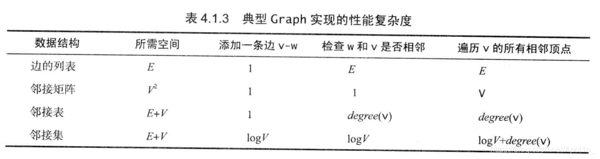
3.1.1 图的表示方式

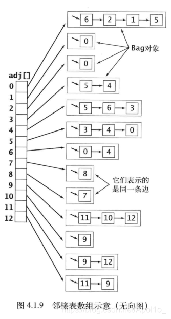
3.1.2 邻接表

将每个顶点的所有相邻顶点都保存在该顶点对应的元素所指向的一张链表中

每条边都会出现两次

• 使用的空间和 V+E 成正比
• 添加 1条边的所需时间为常数
• 遍历顶点v的所有相邻顶点的时间与度数成正比

public class Graph {
    private final int V;//顶点数目
    private int E;//边数目
    private Bag<Integer>[] adj;//邻接表
    public Graph(int V) {
        this.V = V;
        adj = (Bag<Integer>[])new Bag[V];
        for(int v=0; v<V; v++) {
            adj[v] = new Bag<Integer>();
        }
    }
    /**
     * compute V's degree
     */
    public static  int degree(Graph G, int v) {
        int degree = 0;
        for(int w:G.adj(v))    degree++;
        return degree;
    }
    /**
     * cal max(degree(G,v))
     */
    public static int maxDegree(Graph G) {
        int max = 0;
        for(int v=0; v<G.V(); v++) {
            if(degree(G, v) > max)
                max = degree(G, v);
        }
        return max;
    }
    /**
     * 所有节点平均度数
     */
    public static double avgDegree(Graph G) {
        return 2*G.E()/G.V();
    }
    /**
     * 计算环的个数
     */
    public static int numberOfSelfLoops(Graph G) {
        int cnt = 0;
        for(int v=0; v<G.V(); v++) {
            for(int w : G.adj(v)) {
                if(w == v)    cnt++;
            }
        }
        return cnt/2;    //每条边标记过2次
    }
    /**
     * return the num of vetexs
     */
    public int V() {
        return V;
    }
    /**
     * return the num of edges
     */
    public int E() {
        return E;
    }
    /**
     * add a edge bwteen v and w
     */
    public void addEdge(int v, int w) {
        adj[v].add(w);
        adj[w].add(v);
        E++;
    }
    /**
     * all vertexs(array) adjoin v
     */
    public Iterable<Integer> adj(int v){
        return adj[v];
    }
}

3.1.3 深度优先搜索—-DFS

public class DFS {
    private boolean[] marked;
    private int count;
    public DFS(Graph G, int s) {
        marked = new boolean[G.V()];
        dfs(G, s);
    }
    private void dfs(Graph G, int v) {
        marked[v] = true;
        count++;
        for(int w:G.adj(v)) {
            if(!marked[w])    dfs(G, w);//若当前顶点没有走过，go ahead！
        }
    }
    public boolean marked(int w) {
        return marked[w];
    }
    public int count() {
        return count;
    }
}

DFS只需要一个递归方法来遍历所有节点，在访问一个顶点时：

• 标记当前节点：已访问
• 递归的访问该节点所有没有被标记过的邻接点

通常，理解一个算法算好的方法就是跟踪它的行为

我们要注意两点：

1. 算法遍历边和访问顶点的顺序和图的表示是有关的，因为DFS只会访问当前节点所有的相邻极点
2. 每条边都会被访问两次。并且第二次访问时总发现当前节点已经标记过了

3.1.4 寻找路径

我们利用DFS来建立一个寻找路径的算法

public class DFSpaths {
    private boolean[] marked; // 顶点标记数组
    private int[] edgeTo;
    private final int s; // 起点【source】
    public DFSpaths(Graph G, int s) {
        // TODO Auto-generated constructor stub
        marked = new boolean[G.V()];
        edgeTo = new int[G.V()];
        this.s = s;
        dfs(G, s);
    }
    private void dfs(Graph G, int v) {
        marked[v] = true;
        for (int w : G.adj(v)) {
            if (!marked[w]) { // if Vertex w isn't marked
                /**
                 * 到达顶点w的是顶点v
                 */
                edgeTo[w] = v;
                dfs(G, w);
            }
        }
    }
    public boolean hasPathTo(int v) {
        return marked[v];
    }
    public Iterable<Integer> pathTo(int v) {
        /**
         * 如果v没被标记，说明没有顶点能够到顶点v，返回
         */
        if (!hasPathTo(v))
            return null;
        Stack<Integer> path = new Stack<Integer>();
        for (int x = v; x != s; x = edgeTo[x]) { // 从终点向起点走，利用栈保存
            path.push(x);
        }
        path.push(s);
        return path;
    }
}

edgeTo[] 数组会记住每个顶点到起点的路径，从而形成一个以起点s 为根的含有所有与s相连的路径的树

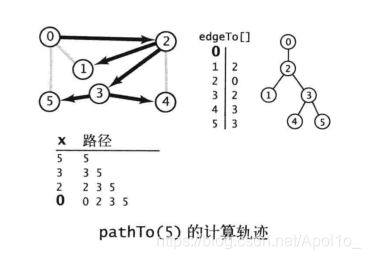
【将DFS的轨迹想象成一个树的构成】

3.1.5 广度优先搜索—BFS

在BFS中，我们希望按照与起点的顺序来遍历所有顶点，看起来很容易实现————使用队列

广度优先搜索的真正目标：————为了找到最短路径

3.1.5.1 实现

算法流程简述：

1. 先将起点 s 加入队列
2. 反复执行下列行为，直至队列空：
   1. 取队列的下一个顶点，并标记它
   2. 将当前顶点的所有（未标记的）邻点都放入队列

BFS算法并不是递归的，它最终也能形成一棵树

public class BFS {
    private boolean[] marked;
    private int[] edgeTo;
    private final int s;    //source
    public BFS(Graph G, int s) {
        marked = new boolean[G.V()];
        edgeTo = new int[G.V()];
        this.s = s;
        bfs(G, s);
    }
    private void bfs(Graph G, int v) {
        Queue<Integer> queue = new Queue<Integer>();//利用队列结构来实现bfs
        marked[v] = true;
        queue.enqueue(v);
        while(!queue.isEmpty()) {
            int t = queue.dequeue();
            for(int w : G.adj(t)) {
                if(!marked[w]) {
                    edgeTo[w] = t;        //到达w的顶点为t
                    marked[w] = true;    //标记已经访问过的顶点
                    queue.enqueue(w);
                }
            }
        }
    }
    public boolean hasPathTo(int v) {
        return marked[v];
    }
    public Iterable<Integer> pathTo(int v) {
        /**
         * 如果v没被标记，说明没有顶点能够到顶点v，返回
         */
        if (!hasPathTo(v))
            return null;
        Stack<Integer> path = new Stack<Integer>();
        for (int x = v; x != s; x = edgeTo[x]) { // 从终点向起点走，利用栈保存
            path.push(x);
        }
        path.push(s);
        return path;
    }
}

同样的，使用BFS算法遍历时，每条边都会被访问两次，且第二次访问时这条边已经被标记过了

3.1.6 DFS和BFS

这两个算法的不同之处仅仅在于从数据结构中获取下一个顶点的规则

• 对于BFS来说，是最早加入的顶点
• 对于DFS来说，是最晚加入的顶点（递归的过程，最早加入的最后才会返回）

3.1.7 连通分量

过程

1. 从0 号顶点开始 dfs 遍历
2. 如果遇到没有标记的顶点，重复进行遍历（遍历的路径上的所有顶点都是一个连通分量）

public class CC {
    private boolean[] marked;
    private int[] id;
    private int count;
    public CC(Graph G) {
        marked = new boolean[G.V()];
        id = new int[G.V()];
        for (int x = 0; x < G.V(); x++) {
            /**
             * 从第一个顶点开始，如果位被标记，则从该节点dfs遍历（一个新的连通分量）
             */
            if (!marked[x]) {
                dfs(G, x);
            }
            count++; // 下一个连通分量
        }
    }
    private void dfs(Graph G, int v) {
        marked[v] = true;
        id[v] = count;
        for (int w : G.adj(v)) {
            if (!marked[w]) {
                /**
                 * 从起点v开始的所有遍历过的路径上的所有顶点都是一个连通分量
                 */
                id[w] = count;
                dfs(G, w);
            }
        }
    }
    public boolean connected(int v, int w) {
        return id[v] == id[w];
    }
    public int id(int v) {
        return id[v];
    }
    public int count() {
        return count;
    }
}

3.1.8 使用DFS的应用

3.1.8.1 判断是否有环

public class Cycle {
    private boolean[] marked;
    private boolean hasCycle;
    public Cycle(Graph G) {
        marked = new boolean[G.V()];
        for(int s=0; s<G.V(); s++) {
            if(!marked[s]) {
                dfs(G, s, s);
            }
        }
    }
    private void dfs(Graph G, int v, int u) {
        marked[v] = true;
        for(int w:G.adj(v)) {
            if(!marked[w]) {
                dfs(G, w, v);
            }
            else if( v == u) {
                /**
                 * dfs的参数为当前顶点和已经标记的相邻顶点，如果两个顶点相等，说明遇到了环
                 */
                hasCycle = true;
                     break;
            }
        }
    }
    public boolean haCycle() {
        return hasCycle;
    }
}

3.1.8.2 是否为二分图（双色问题）

public class TwoColor {
    private boolean[] marked;
    private boolean[] color;
    private boolean isTwocolor = true;
    public TwoColor(Graph G) {
        marked = new boolean[G.V()];
        color = new boolean[G.V()];;
        for (int s = 0; s < G.V(); s++) {
            if (!marked[s]) {
                dfs(G, s);
            }
        }
    }
    private void dfs(Graph G, int v) {
        marked[v] = true;
        for (int w : G.adj(v)) {
            if (!marked[v]) {
                color[w] = !color[v];//在遍历下一个顶点之前做动作
                dfs(G, w);
            } else if (color[v] == color[w]) // 如果两个相邻顶点颜色一样，则不是二分图
                isTwocolor = false;
        }
    }
    public boolean isTwoColor() {
        return isTwocolor;
    }
}

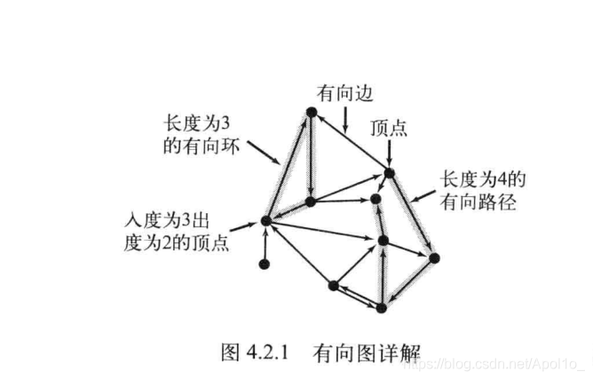
3.2. 有向图

3.2.1 基本API实现

public class Digraph {
    private final int V;//顶点数目
    private int E;//边数目
    private Bag<Integer>[] adj;//邻接表
    public Digraph(int V) {
        this.V = V;
        adj = (Bag<Integer>[])new Bag[V];
        for(int v=0; v<V; v++) {
            adj[v] = new Bag<Integer>();
        }
    }
    /**
     * return the num of vetexs
     */
    public int V() {
        return V;
    }
    /**
     * return the num of edges
     */
    public int E() {
        return E;
    }
    /**
     * add an edge bwteen v and w
     * notice that in the Digraph, every edges have a direction 
     */
    public void addEdge(int v, int w) {
        adj[v].add(w);//因为是有向的，所以只需要添加一条边
        E++;
    }
    /**
     * all vertexs(array) adjoin v
     */
    public Iterable<Integer> adj(int v){
        return adj[v];
    }
    /**
     * 构造有向图的反向图
     */
    public Digraph reverse() {
        Digraph R = new Digraph(V);
        for(int v=0; v<V; v++) {
            for(int w:adj(v)) {
                R.addEdge(w, v);
            }
        }
        return R;
    }
}

3.2.2 DFS、BFS

本质上和无向图的DFS、BFS实现是一样的（同样的思想）

3.2.3 多点可达性

给定一副有向图和顶点的集合，回答：

• 是否存在一条从集合中的任意顶点到达给定顶点v的有向路径

实际应用：内存管理系统(java垃圾回收机制)

3.2.4 调度问题

一种应用广泛的模型是给定一组任务并安排执行顺序

最重要的一种限制条件————优先级限制

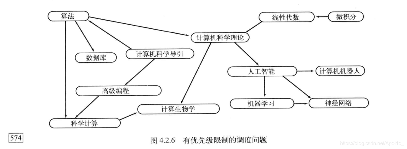
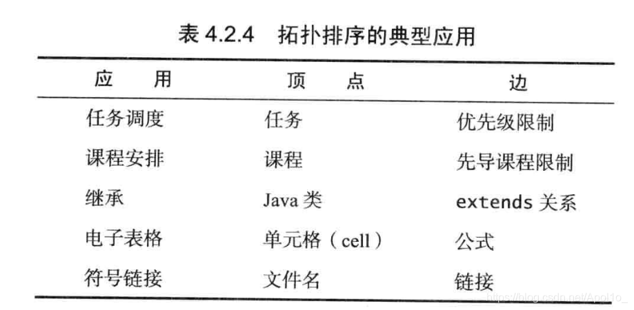
3.2.5 拓扑排序

优先级限制下的调度问题 等价于 拓扑排序问题

【拓扑排序】：给定一副有向图，将所有的顶点排序，使得所有的有向边均从排在前面的元素指向排在后面的元素

拓扑排序（或者说优先级限制问题）是针对有向无环图【DAG】的，因此是不允许有环的

拓扑排序就是dfs逆后序的顶点排序

3.2.6 有向图寻找环

寻找环的基本思想还是利用DFS算法，

但是我们增加了一个boolean类型的数组onStack[]来保存递归调用期间栈上的所有顶点

如果找到一条边v->w，并且w已在栈中（也就意味着之前已经标记过的顶点w在之后又被找到，也就是一条环路）

则找到了一个有向环

public void dfs(Digraph G, int s) {
        marked[s] = true;
        onStack[s] = true;
        for(int w:G.adj(s)) {
            if(hasCycle())    return;
            else if(!marked[w]) {
                edgeTo[w] = s;
                dfs(G, w);
            }
            else if(onStack[w]) {//有环路，则记录环路路径
                cycle = new Stack<Integer>();
                cycle.push(w);
                for(int x=edgeTo[w]; x != w; x = edgeTo[x]) {
                    cycle.push(x);
                }
            }
            onStack[s] = false; //若当前搜索路径没有找到环，需要将栈数组复原，以便下一条路径的搜索
        }
    }

3.2.7 强连通性

如果一副有向图中的任意两个顶点都是强连通的，则称这幅图是强连通的

（难以理解，跳过，后续深入）

3.2.8 顶点对的可达性

只需利用DFS进行可达性的判定，但无法使用于大型图网络（构造图的代价太高）

public class TransitiveClosure {
    private DirectedDFS[] all;
    public TransitiveClosure(Digraph G) {
        all = new DirectedDFS[G.V()];//有向图DFS
        for(int v=0; v<G.V(); v++) {
            /**
             * 构造了一个二维数组，相当于矩阵表示图关系
             * 每个节点DFS一次，若v和w相连，那么marked[w]一定为true
             */
            all[v] = new DirectedDFS(G, v);
        }
    }
    public boolean reachable(int v, int w) {
        return all[v].marked(w);
    }
}

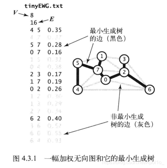
3.3. 最小生成树

给定一副加权无向图，找到它的一棵最小生成树

图的生成树是它的一棵含有其所有顶点的无环连通子图。

最小生成树【MST】是一棵权值之和最小（成本最小）的生成树。

3.3.1 一些约定

• 只考虑连通图
• 边的权重不一定表示距离
• 边的权重可能是0或者负数
• 所有边的权重各不相同

3.3.2 原理

反证法

3.3.3 切分定理下的贪心算法

切分定理是解决最小生成树问题的所有算法的基础

这些都是贪心算法的特殊情况：使用切分定理找到最小生成树的一条边，不断重复直到找到所有边

一棵树【tree】的特点：V个顶点有V-1条边

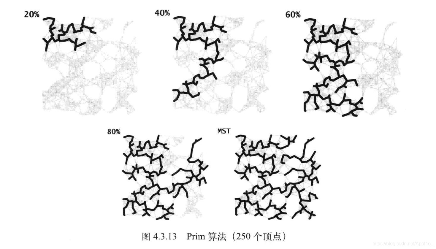
3.3.4 Prim算法

数据结构

• 顶点：marked[]数组
• 边：Edge对象
• 横切边：最小优先队列MinPQ

3.3.4.1 延时实现

每当我们向树中添加了一条边之后，也向树中添加了一个顶点

将连接这个顶点和其他不再树中顶点的边加入优先队列

两端顶点都在树中的边已经失效了（防止环的出现）

延时的实现会将失效的边留在优先队列里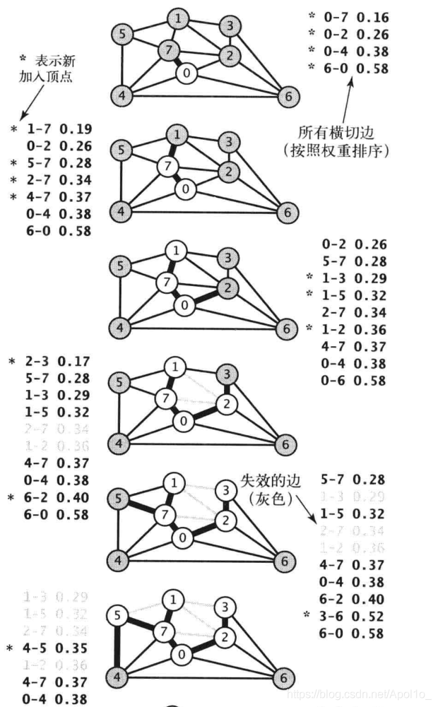

在添加了V个顶点之后（V-1条边），最小生成树就完成了

（优先队列中余下的项都是无效的，不需要再检查它们）

public class LazyPrimMST {
    private boolean[] marked;//顶点
    private Queue<Edge> mst;//边
    private MinPQ<Edge> pq;//横切边（包括最小的边）
    public LazyPrimMST(EdgeWeightedGraph G) {
        marked = new boolean[G.V()];
        mst = new Queue<Edge>();
        pq = new MinPQ<Edge>();
        visit(G, 0);
        while(!pq.isEmpty()) {
            Edge e = pq.delMin();    //找到最小横切边
            int v = e.either();
            int w = e.other(v);
            /**
             *    忽略无效边（形成环的边） 
             */
            if(marked[v] && marked[w])    continue;
            mst.enqueue(e);//最小生成树加入边
            /**
             * 访问未标记的顶点，将边放入优先队列中
             */
            if(!marked[v])    visit(G, v);
            if(!marked[w])    visit(G, w);
        }
    }
    /**
     * 将顶点v连接的边加入优先队列中
     */
    private void visit(EdgeWeightedGraph G, int v) {
        marked[v] = true;
        for(Edge w:G.adj(v)) {
            if(!marked[w.other(v)]) {    //如果当前边没有被添加过【两个顶点未被全部标记】
                pq.insert(w);
            }
        }
    }
    public Iterable<Edge> mst(){
        return mst;
    }
    /**
     * 延迟计算权重
     */
    public double weight() {
        double w = 0;
        for(int i=0; i<marked.length-1; i++) {
            Edge e = mst.dequeue();
            w += e.weight();
            mst.enqueue(e);
        }
        return w;
    }
}

3.3.4.2 即时实现

基本思路是：

• 从一个根节点出发，每一个找到一条与当前树相连（且不在树中）的权值最小的边(也就是最短的横切边)
• 将该边加入树中
• 反复执行该过程，直到N个顶点全部被标记完成

顶点索引的edgeTo[]和distTo[]数组

它们具有如下性质：

1. 如果顶点v不在树中，但是至少一条边和树相连，那么edgeTo[v]是与v相连的最短的边，distTo[v]为该边的权重
2. 所有的这类顶点v都保存在最小优先队列中

算法处理的过程：

• 首先从优先队列中取出权值最小的边
• 检查每条边v—w，如果w已经标记过了，则什么也不做
• 否则， 如果当前边已经存在与优先队列中并且小于当前队列中的数值，更新它的值（说明到w点还有距离更短的边）
• 如果不在优先队列中，添加它
  

【思考】

为什么每次都能找到与当前树相连的权重最小的边呢？————优先队列

public class PrimMST {
    private Edge[] edgeTo; // 距离当前树权重最小的边
    private double[] distTo;// weight[w] = edgeTo[w].weight()
    private boolean[] marked;// 如果v在树种则为true
    private IndexMinPQ<Double> pq;// 有效边的横切边
    public PrimMST(EdgeWeightedGraph G) {
        edgeTo = new Edge[G.V()];
        distTo = new double[G.V()];
        marked = new boolean[G.V()];
        pq = new IndexMinPQ<Double>(G.V());
        for (int v = 0; v < G.V(); v++) {
            distTo[v] = Double.POSITIVE_INFINITY;
        }
        distTo[0] = 0.0;
        pq.insert(0, 0.0); // 初始化最小优先队列
        while (!pq.isEmpty()) { // 将与树相连的最小权重边加入树中
            visit(G, pq.delMin());
        }
    }
    /**
     * 将顶点加到树中，更新数据
     */
    private void visit(EdgeWeightedGraph G, int v) {
        marked[v] = true;
        for (Edge e : G.adj(v)) {
            if (marked[e.other(v)])
                continue; // 一条边的两个顶点都被标记过，则什么也不做
            if (e.weight() < distTo[e.other(v)]) {//如果当前边小于优先队列中到这个点的距离
                edgeTo[e.other(v)] = e;
                distTo[e.other(v)] = e.weight();
                if (pq.contains(e.other(v))) {//若不再优先队列中，添加进去
                    pq.changeKey(e.other(v), distTo[e.other(v)]);
                } else {//否则，更新它
                    pq.insert(e.other(v), e.weight());
                }
            }
        }
    }
}

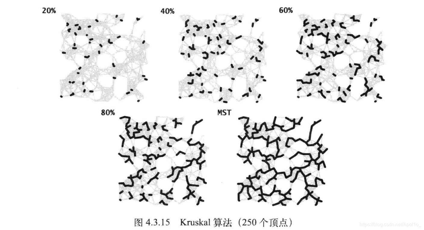
3.3.5 Kruskal算法

将边按照权重排序

依次选择权重最小的边加入（前提：不形成环）

选择的边由森林逐渐形成树

Prim是由一条边一条边地构成一棵树，从一个根节点开始，每一步不断添加一条边

Kruskal是由不同的边，它的边会连接成森林，最终连成一棵树

public class KruskalMST {
    private Queue<Edge> mst;
    public KruskalMST(EdgeWeightedGraph G) {
        mst = new Queue<Edge>();
        MinPQ<Edge> pq = new MinPQ<Edge>((Comparator<Edge>) G.edges());
        UF uf = new UF(G.V());
        while (mst.size() < G.V() - 1 && !pq.isEmpty()) {
            Edge e = pq.delMin(); // 找到权重最小的边
            int v = e.either();
            int w = e.other(v);
            if (uf.connected(v, w))
                continue; // 如果在找到一条边的两个端点已经在一个连通分量上，说明这条边的连接必定会形成环
            uf.union(v, w);
            mst.enqueue(e);
        }
    }
}

Kruskal算法比Prim算法要慢一些，两个算法都需要对每条边进行优先队列操作

Kruskal算法还需要进行依次union操作（连接两个点形成一个连通分量）

3.4. 最短路径

3.4.1 定义

从顶点s到顶点t的最短路径是所有从s到t的路径中权重最小的

3.4.2 性质

• 路径是有向的
• 并不是所有顶点都是可达的
• 负权重会使问题变复杂
• 最短路径一般都是简单图
• 最短路径不一定是唯一的
• 可能存在平行边和自环

3.4.3 最短路径树

最短路径问题，最后会给出一个根节点为起点s的最短路径树，它包含了s到所有可达顶点的最短路径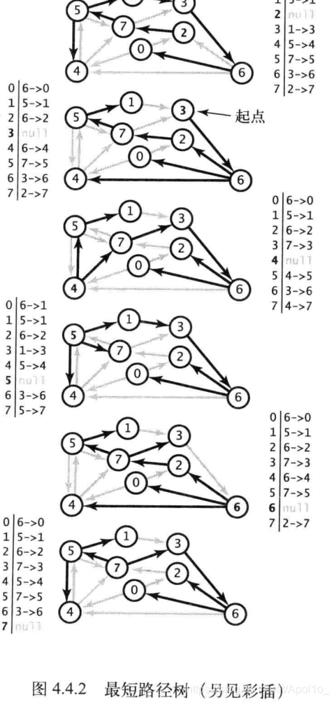

3.4.4 有向加权边API

public class DirectedEdge {
    private final int v; // 顶点之一
    private final int w; // 另一个顶点
    private final double weight; // 权重
    public DirectedEdge(int v, int w, double weight) {
        this.v = v;
        this.w = w;
        this.weight = weight;
    }
    public double weight() {
        return weight;
    }
    public int from() {
        return v;
    }
    public int to() {
        return w;
    }
}

3.4.5 有向加权图API

public class EdgeWeightedDigraph {
    private final int V;// 顶点总数
    private int E;// 边总数
    private Bag<DirectedEdge>[] adj;// 邻接表
    public EdgeWeightedDigraph(int V) {
        this.V = V;
        adj = (Bag<DirectedEdge>[]) new Bag[V];
        for (int v = 0; v < V; v++) {
            adj[v] = new Bag<DirectedEdge>();
        }
    }
    public int V() {
        return V;
    }
    public int E() {
        return E;
    }
    public void addEdge(DirectedEdge e) {
        adj[e.from()].add(e);// 有向图，只需要加入一条边
        E++;
    }
    public Iterable<DirectedEdge> adj(int v) {
        return adj[v];
    }
    /**
     * 返回加权有向图的所有边
     */
    public Iterable<DirectedEdge> edges() {
        Bag<DirectedEdge> b = new Bag<DirectedEdge>();
        for (int v = 0; v < V; v++) {
            for (DirectedEdge e : adj[v]) {
                b.add(e);
            }
        }
        return b;
    }
}

不同于无向图，在加权有向图中，每条边在邻接表中仅出现一次

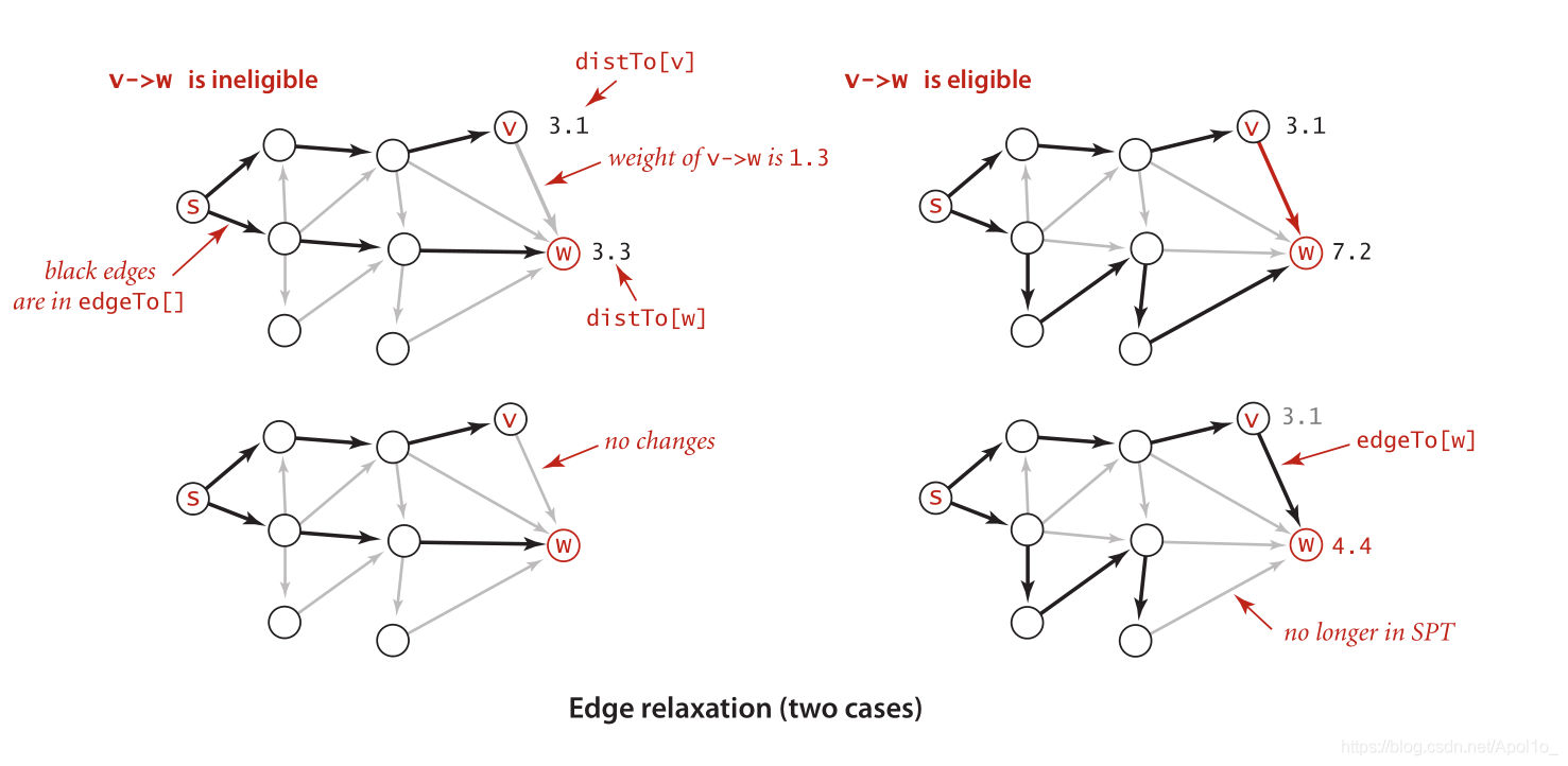
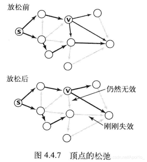
3.4.6 边的松弛【relax】

我们的最短路径算法的实现都是基于一个叫做松弛【relax】的操作进行的

在遇到新的边v——>w时，需要进行松弛操作：

• 如果dist[w] <= dist[v] + e.weight()：
  则说明到s到w的路径和不大于从s到v再从v到w的路径和，那么v——>w这条边就失效了（不选择这条边）
• 如果dist[w] > dist[v] + e.weight()：
  更新dist[w]的值

/*
    边的松弛
*/
public void relax(DirectedEdge e){
    int v = e.from();
    int w = e.to();
    if(dist[v] + e.weight() < dist[w]){
        dist[w] = dist[v] + e.weight();    //更新成更小的权重和
        edgeTo[w] = e;    //更新到w的边，之前的边会被替换为新边e
    }
}

放松一条边就类似于：

将橡皮筋转移到一条更短的路径上，从而放松了较长边的压力

3.4.7 顶点的松弛

对于每一个顶点，我们会遍历所有顶点的邻边，并对所有邻接边进行松弛操作

因为，在最短路径中，每一个顶点有且只有一条边连接到它（前提：从源点可达）

/*
    顶点的松弛
*/
public void relax(EdgeWeightedDigraph G, int v){
    for(DirectedEdge e : G.adj[v]){
        int w = e.to();
        if(dist[w] > dist[v] + e.weight()){
            dist[w] = dist[v] + e.weight();    //更新成更小的权重和
            edgeTo[w] = e;    //更新到w的边，之前的边会被替换为新边e
        }
    }
}

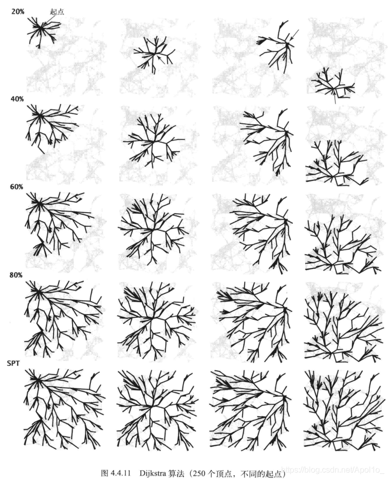
3.4.9 Dijkstra算法

回忆一下Prim算法：每一次向树中添加一条边

Dijkstra算法也是采用了类似的方法

• 首先将dist[s]初始化为0
• dist[]中其他的元素初始化为正无穷（即不可达）
• 然后将dist[]中最小的非树顶点进行松弛操作，并加入树中
• 如此这般直到所有顶点都在树中，或者非树顶点为正无穷（即完成算法，或者某些顶点不可达）

另外，dijkstra算法在对边的松弛时，需要处理两种情况：

1. 如果边的to()不在优先队列中，添加进pq
2. 如果已在优先队列中，需要降低优先级

3.4.9.1 实现

public class DijkstraSP {
    private DirectedEdge[] edgeTo;
    private double[] distTo;
    private IndexMinPQ<Double> pq;
    public DijkstraSP(EdgeWeightedDigraph G, int s) {
        edgeTo = new DirectedEdge[G.V()];
        distTo = new double[G.V()];
        pq = new IndexMinPQ<Double>(G.V());
        //将所有边到起点的距离初始化为正无穷
        for (int v = 0; v < G.V(); v++) {
            distTo[v] = Double.POSITIVE_INFINITY;
        }
        distTo[s] = 0.0;
        pq.insert(s, 0.0);
        while(!pq.isEmpty()) {
            relax(G, s);//对所有顶点进行松弛操作
        }
    }
    /**
     * 顶点的松弛操作
     * 1. 如果边的to()不在优先队列中，添加进pq
     * 2. 如果已在优先队列中，需要降低优先级
     */
    private void relax(EdgeWeightedDigraph G, int v) {
        for(DirectedEdge e : G.adj(v)){
            int w = e.to();
            if(distTo[w] > distTo[v] + e.weight()){
                distTo[w] = distTo[v] + e.weight();    //更新成更小的权重和
                edgeTo[w] = e;    //更新到w的边，之前的边会被替换为新边e
                if(pq.contains(w))    pq.change(w, e.weight());
                else    pq.insert(w, e.weight());
            }
        }
    }
}

dijkstra算法是每一次往树中添加一条边，该边是由树中的顶点指向非树中的顶点w，且是到s最近的点

该算法可以找到给定两点的最短路径

3.4.9.2 时间复杂度

在一副有V个顶点和E条边的加权有向图，时间与ElogV成正比（最坏情况下）

但是，对于有负权重的加权有向图中的最短路径问题，dijkstra算法无法完成这类问题

【问题】：（未答）

为什么dijkstra算法无法解决带负权重问题呢？

3.4.10 无环加权有向图的最短路径算法

特点：

• 能够在线性时间解决单点最短路径
• 能够处理负权重的边
• 能够解决相关的问题，例如找出最长的路径

只要将顶点的放松和拓扑排序结合起来，马上就能够得到一种解决无环加权有向图中的最短路径的算法

3.4.11 解决负权重的最短路径算法

Bellman-ford算法

时间复杂度#card=math&code=O%28VE%29&id=ilkEE)

（后续跟进）